TAI BUI
Back to curriculum
BuildPython

Proximal Policy Optimization (PPO)

A2C throws away each rollout after one update. PPO wraps the policy gradient in a clipped importance ratio, so you can run 10+ epochs on the same data without the policy exploding. Schulman et al. (2017). Still the default policy-gradient algorithm in 2026.

TIME: ~75 minutesPREREQUISITES: Phase 9 · 06 (REINFORCE), Phase 9 · 07 (Actor-Critic)

Learning Objectives

  • Explain why PPO clips the importance ratio r_t(θ) instead of enforcing TRPO's hard KL trust-region constraint.
  • Implement the clipped surrogate objective and the full PPO loss (surrogate plus value loss plus entropy bonus) from scratch, including the multi-epoch training loop.
  • Diagnose a PPO run's health from mean KL, clip fraction, and explained variance, and know what to change when each one drifts out of range.
  • Place PPO's clipped-surrogate design relative to its 2026 variants (GRPO, DPO, KL-penalty RLHF) and name the pitfalls most likely to break an implementation.

The Problem

A2C (Lesson 07) is on-policy: the gradient E_{π_θ}[A · ∇ log π_θ] needs data sampled from the current π_θ. Take one update and π_θ changes, so the data you just collected is already off-policy. Reuse it and the gradient is biased.

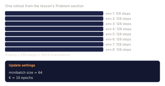
Rollouts aren't free, either. On Atari, one rollout across 8 envs × 128 steps works out to 1024 transitions and a dozen seconds of environment time. Throwing all of that away after a single gradient step is wasteful.

Trust Region Policy Optimization (TRPO, Schulman 2015) was the first real fix: constrain each update so the KL divergence between the old and new policy stays below some δ. Theoretically clean, but it needs a conjugate-gradient solve per update. Nobody runs TRPO in 2026.

PPO (Schulman et al. 2017) swaps the hard trust-region constraint for a simple clipped objective. One extra line of code. Ten epochs per rollout. No conjugate gradients. Guarantees that are good enough in practice. Nine years later, it's still the default policy-gradient algorithm for everything from MuJoCo to RLHF.
Warm-up0/3
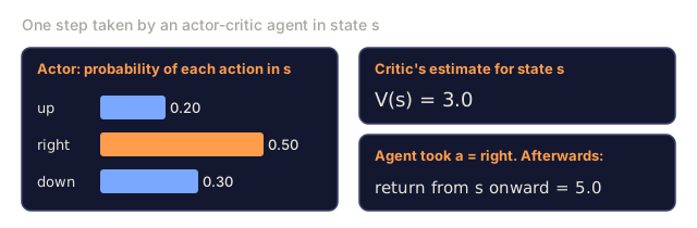
1. In actor-critic methods such as A2C, what does the advantage A(s, a) tell you?Warm-up
An actor-critic agent in state s: the actor gives probabilities up 0.20, right 0.50 and down 0.30, the agent took right, the critic estimates V(s) = 3.0, and the return observed from s onward was 5.0.
Illustrative numbers.
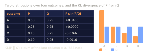
2. What does the KL divergence between two probability distributions measure?Warm-up
Two distributions P (0.50, 0.25, 0.15, 0.10) and Q (0.25 each) over outcomes A to D as paired bars, with a table of P x ln(P/Q) per outcome and a total KL(P || Q) of 0.1783 nats.
Worked by hand from the KL formula.
3. What does adding an entropy bonus to a policy-gradient loss encourage?Warm-up
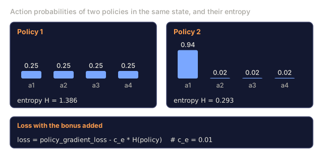
Bars for two policies over four actions: policy 1 has 0.25 on each, policy 2 has 0.94, 0.02, 0.02 and 0.02; their entropies are 1.386 and 0.293. Below, a loss line with a c_e times entropy term, c_e = 0.01.
Entropy computed from the probabilities.
Check: The Problem0/2
1. Why can A2C not simply run several gradient steps on one rollout?Explain
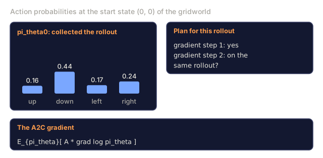
Four bars for the gridworld's start state giving action probabilities (up, down, left, right) under the policy that collected a rollout, a card asking whether a second gradient step on the same rollout is possible, and the A2C gradient expression.
Probabilities are real: lesson's code after five updates.
2. Why does the lesson say nobody runs TRPO in 2026 despite its clean theory?Explain
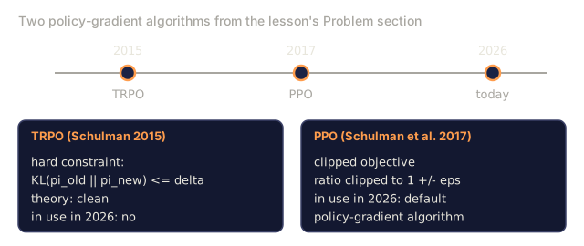
A timeline marking TRPO in 2015, PPO in 2017 and today in 2026, above two cards: TRPO with a hard KL constraint, clean theory and not used in 2026, and PPO with a clipped objective, used as the default policy-gradient algorithm in 2026.
Facts from the lesson text.

The Concept

PPO clipped surrogate objective: ratio clipping at 1 ± ε

The importance ratio.

r_t(θ) = π_θ(a_t | s_t) / π_{θ_old}(a_t | s_t)

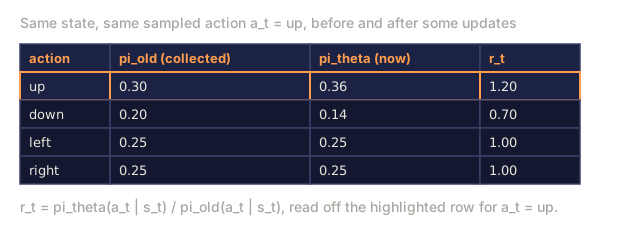
This is the likelihood ratio of the new policy versus the policy that collected the data. r_t = 1 means no change. r_t = 2 means the new policy is twice as likely to take a_t as the old one.

The clipped surrogate.

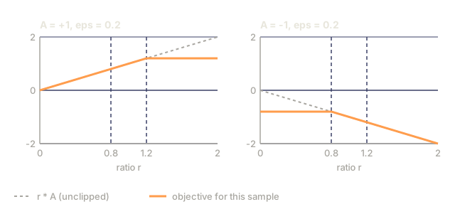
L^{CLIP}(θ) = E_t [ min( r_t(θ) A_t, clip(r_t(θ), 1-ε, 1+ε) A_t ) ]

Two terms:

  • If the advantage A_t > 0 and the ratio tries to grow past 1 + ε, the clip flattens the gradient: don't push a good action further than +ε above old probability.
  • If the advantage A_t < 0 and the ratio tries to grow past 1 - ε (meaning we would make a bad action more likely compared to its clipped reduction), the clip caps the gradient: don't push a bad action below -ε.

The min handles the other direction: if the ratio has already moved in the beneficial direction, you still get the gradient (no clipping on the side that would hurt you).

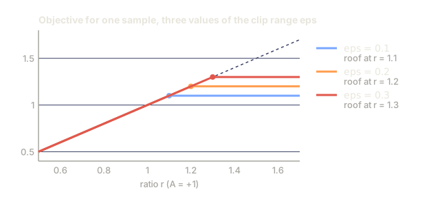
Typical ε = 0.2. Plot the objective as a function of r_t and you get a piecewise-linear curve, flat on the roof for the good side and flat on the floor for the bad side.

The full PPO loss.

L(θ, φ) = L^{CLIP}(θ) - c_v · (V_φ(s_t) - V_t^{target})² + c_e · H(π_θ(·|s_t))

Same actor-critic structure as A2C. Three coefficients, usually c_v = 0.5, c_e = 0.01, ε = 0.2.

The training loop.

  1. Collect N × T transitions across N parallel envs for T steps each.
  2. Compute advantages (GAE), freeze them as constants.
  3. Freeze π_{θ_old} as a snapshot of current π_θ.
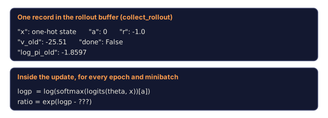
  4. For K epochs, for each minibatch of (s, a, A, V_target, log π_old(a|s)):
    • Compute r_t(θ) = exp(log π_θ(a|s) - log π_old(a|s)).
    • Apply L^{CLIP} + value loss + entropy.
    • Gradient step.
  5. Discard the rollout. Return to step 1.

K = 10 and minibatches of 64 make a standard hyperparameter set. PPO doesn't fuss over the exact numbers: they rarely matter within ±50%.

KL-penalty variant. The original paper also proposed an adaptive KL penalty as an alternative: L = L^{PG} - β · KL(π_θ || π_old), with β adjusted based on observed KL. The clipping version won out; the KL variant survives in RLHF, where KL to the reference policy is already a constraint you want anyway.
Check: The Concept0/13
1. What does the importance ratio r_t(θ) = π_θ(a_t|s_t) / π_old(a_t|s_t) measure?Define
A table for one state with four actions giving the probability under the data-collecting policy, under the current policy, and their quotient: up 0.30 to 0.36 gives 1.20, down 0.20 to 0.14 gives 0.70, left and right stay at 0.25 giving 1.00; the up row is highlighted as the sampled action.
Illustrative probabilities.
2. What is PPO's clipped surrogate?Define
Two plots of one sample's objective against the ratio r from 0 to 2 with eps = 0.2: for advantage +1 and for advantage -1, each showing the dashed line r*A and a solid curve for the sample's objective, with dotted verticals at 0.8 and 1.2.
Solid curve computed from the lesson's formula.
3. What is a trust region in TRPO and PPO?Define
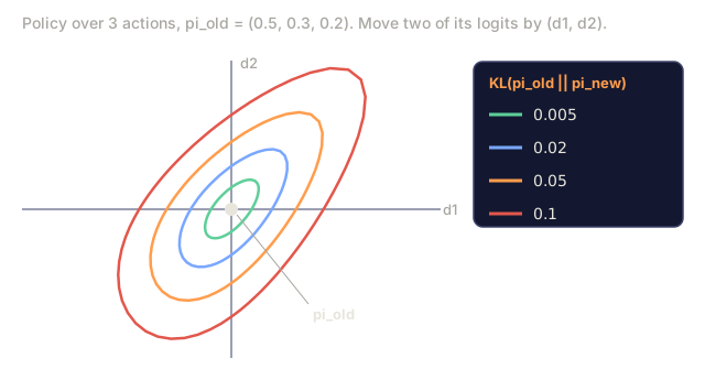
Contour plot in a two-dimensional slice of logit space for a three-action softmax policy with probabilities 0.5, 0.3, 0.2: four closed curves around the old policy mark where KL from the old policy equals 0.005, 0.02, 0.05 and 0.1.
Computed with numpy: KL(pi_old || pi_new) as two logits move.
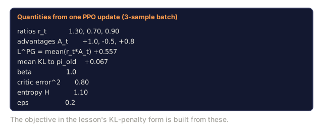
4. What is the KL-penalty form of PPO's objective?Define
A card of quantities logged in one PPO update: three ratios, three advantages, L^PG +0.557, mean KL +0.067, beta 1.0, squared critic error 0.80, entropy 1.10 and eps 0.2.
Ratios, advantages, beta, critic error and entropy are illustrative. L^PG and mean KL are computed from the ratios and advantages (per-sample KL taken as -ln r).
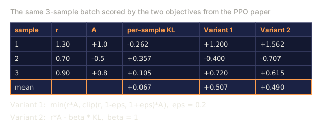
5. Which description fits PPO-KL, 'the other PPO'?Define
A table scoring three samples (ratios 1.30, 0.70, 0.90 with advantages +1.0, -0.5, +0.8) under two objectives: Variant 1 is the clipped surrogate with eps 0.2 and Variant 2 is r*A minus beta times KL with beta 1, with means in the last row.
Computed with numpy; per-sample KL taken as -ln r.
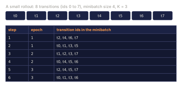
6. What is multi-epoch training in PPO?Define
A rollout of 8 transitions t0 to t7 and a six-row log of gradient steps with minibatch size 4 and K = 3: each epoch shuffles the ids and forms two minibatches, so every transition appears once per epoch across epochs 1, 2 and 3.
Small sizes for illustration; shuffles are random.
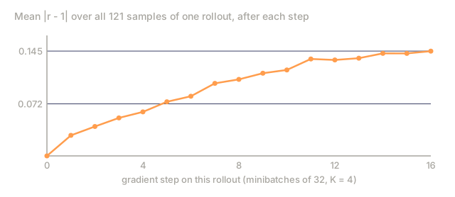
7. Why is PPO called 'on-policy-ish'?Define
Line plot of the mean absolute distance of the importance ratio from 1 over one rollout of 121 samples, starting at exactly 0 before the first step and rising over 16 minibatch steps to 0.145.
Measured by running the lesson's ppo_update loop on one gridworld rollout.
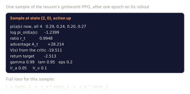
8. What are the three terms of PPO's full loss, and what are the usual starting values of c_v and c_e?Define
A card of one gridworld sample after one epoch: the four action probabilities, log pi_old, the ratio, the advantage, the critic's value, the return target, gamma, lambda, eps and the two learning rates, above a loss line L = term_1 + c_v * term_2 + c_e * term_3 with the terms left unnamed.
Numbers from a real run of the lesson's code; the loss line is the stem's skeleton, not computed.
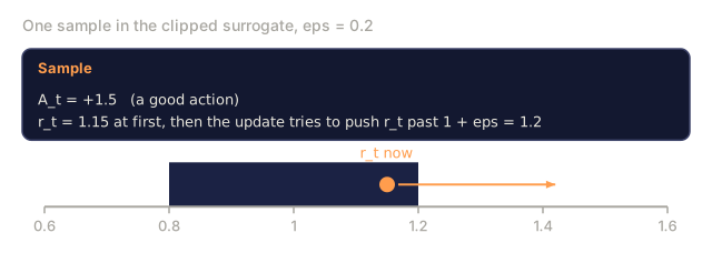
9. In the clipped surrogate, what happens when A_t > 0 and the ratio tries to grow past 1+ε?Explain
A card describing one sample with advantage +1.5 and ratio 1.15 under eps = 0.2, and a number line of the ratio from 0.6 to 1.6 with a shaded band from 0.8 to 1.2, a dot at 1.15 and an arrow pointing right past 1.2.
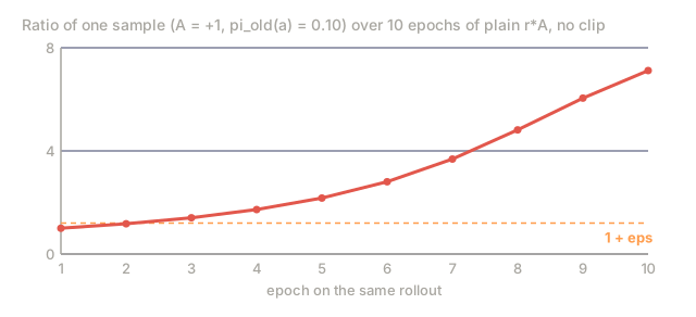
10. Why does clipping let PPO run many epochs on one rollout without the policy exploding?Explain
Plot of the importance ratio of one positive-advantage sample over ten epochs of gradient ascent on the plain r*A objective, rising from 1 to about 7.1, with a dashed horizontal line at 1.2.
Computed: softmax over 4 actions, one sample repeated each epoch, step size 0.15 (illustrative).
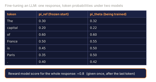
11. Why does the KL-penalty variant of PPO survive in RLHF?Explain
A table of seven tokens of one response, with each token's probability under a frozen reference model and under the policy being trained, followed by a single reward-model score of +0.8 for the whole response.
Illustrative numbers.
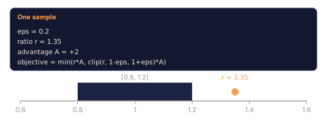
12. With ε = 0.2, ratio r = 1.35 and advantage A = +2, what does min(r·A, clip(r, 1-ε, 1+ε)·A) evaluate to?Apply
A card with eps = 0.2, ratio 1.35, advantage +2 and the min(r*A, clip(r, 1-eps, 1+eps)*A) formula, above a number line from 0.6 to 1.6 with a shaded band from 0.8 to 1.2 and a dot at 1.35.
13. A rollout gives 1024 transitions. With minibatches of 64 and K = 10 epochs, how many gradient steps does one rollout produce?Apply
Eight bars labelled env 1 to env 8, each 128 steps long, totalling 1024 transitions, above a card with minibatch size 64 and K = 10 epochs.
Sizes from the lesson text.

Build It

Step 1: capture log π_old(a | s) at rollout time

python
for step in range(T):
    probs = softmax(logits(theta, state_features(s)))
    a = sample(probs, rng)
    s_next, r, done = env.step(s, a)
    buffer.append({
        "s": s, "a": a, "r": r, "done": done,
        "v_old": value(w, state_features(s)),
        "log_pi_old": log(probs[a] + 1e-12),
    })
    s = s_next

The snapshot gets taken once, at rollout time, and it doesn't change during the update epochs.

Step 2: compute GAE advantages (Lesson 07)

Same as A2C. Normalize across the batch.

Step 3: clipped surrogate update

python
for _ in range(K_EPOCHS):
    for mb in minibatches(buffer, size=64):
        for rec in mb:
            x = state_features(rec["s"])
            probs = softmax(logits(theta, x))
            logp = log(probs[rec["a"]] + 1e-12)
            ratio = exp(logp - rec["log_pi_old"])
            adv = rec["advantage"]
            surrogate = min(
                ratio * adv,
                clamp(ratio, 1 - EPS, 1 + EPS) * adv,
            )
            # backprop -surrogate, add value loss, subtract entropy
            grad_logpi = onehot(rec["a"]) - probs
            if (adv > 0 and ratio >= 1 + EPS) or (adv < 0 and ratio <= 1 - EPS):
                pg_grad = 0.0  # clipped
            else:
                pg_grad = ratio * adv
            for i in range(N_ACTIONS):
                for j in range(N_FEAT):
                    theta[i][j] += LR * pg_grad * grad_logpi[i] * x[j]

The "clipped → zero gradient" pattern is the heart of PPO: once the new policy has drifted too far in the beneficial direction, the update simply stops.

Step 4: value and entropy

Add standard MSE to the critic target and an entropy bonus on the actor, same as A2C.

Step 5: diagnostics

Three things to watch every update:

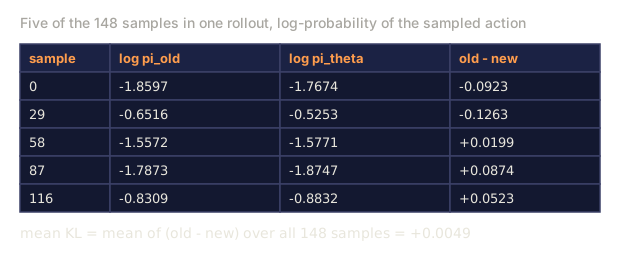
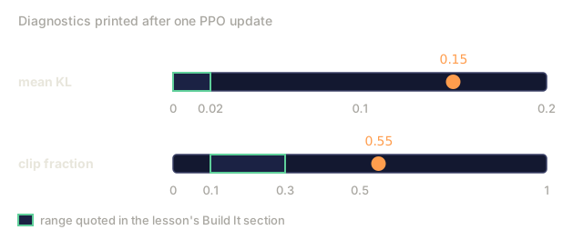
  • Mean KL E[log π_old - log π_θ]. Should stay in [0, 0.02]. If it blows past 0.1, reduce K_EPOCHS or LR.
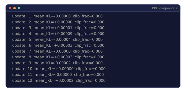
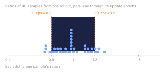
  • Clip fraction: the fraction of samples whose ratio lies outside [1-ε, 1+ε]. Should be ~0.1-0.3. If ~0, the clip never triggers, so raise LR or K_EPOCHS. If ~0.5+, you're over-fitting the rollout, so lower them.
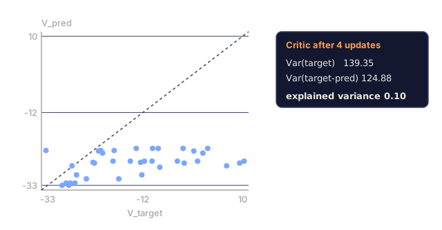
  • Explained variance 1 - Var(V_target - V_pred) / Var(V_target). Critic quality metric. Should climb toward 1 as the critic learns.
Check: Build It0/10
1. What does the clip fraction measure?Define
A number line of the importance ratio from 0.4 to 1.8 with a shaded band between 0.8 and 1.2 and 40 dots, one per sample of a gridworld rollout, stacked where they coincide.
Ratios measured with the lesson's code after two epochs on one rollout.
2. What does explained variance measure in PPO diagnostics, and how should it behave?Define
Scatter of the critic's prediction against its value target for 36 samples of a gridworld rollout, with a dashed diagonal and a card giving the variances and an explained variance of 0.10.
Critic and targets from the lesson's code after four updates.
3. Your PPO run's clip fraction has sat near 0 for a dozen updates. What range should you aim for?Explain
A terminal listing of a PPO run's logged diagnostics for updates 1 to 12, with mean_KL values of 0.00000 or within a few hundred-thousandths of it and clip_frac 0.000 on every line.
Real output of the lesson's code on the gridworld (settings not shown).
4. What mean KL range signals a healthy PPO update, and what do you do if it passes 0.1?Explain
A table of five samples, labelled by their index in a rollout of 148, giving the log-probability of the sampled action under the old and the current policy and their difference, with the mean of the differences over all 148 samples, +0.0049, written as the mean KL.
Real numbers from the lesson's code, one epoch after a rollout; only five of the samples are shown.
5. Why is log π_old stored once at rollout time instead of being recomputed during the update epochs?Explain
A rollout-buffer record with fields x, a, r, done, v_old and log_pi_old (value -1.8597), above the update's ratio line, ratio = exp(logp - ???), with the subtracted term left as question marks.
Record taken from a real rollout of the lesson's code.
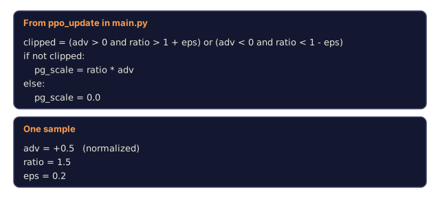
6. In ppo_update, a sample has normalized advantage +0.5, ratio 1.5 and eps = 0.2. What is pg_scale for it?Apply
The five lines of ppo_update that set clipped and pg_scale, above a card for one sample with normalized advantage +0.5, ratio 1.5 and eps 0.2.
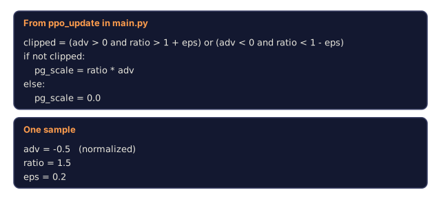
7. In ppo_update, a sample has normalized advantage -0.5, ratio 1.5 and eps = 0.2. What is pg_scale for it?Apply
The five lines of ppo_update that set clipped and pg_scale, above a card for one sample with normalized advantage -0.5, ratio 1.5 and eps 0.2.
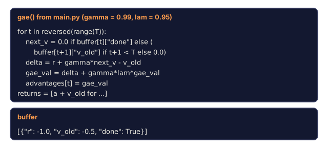
8. In gae(), the buffer holds one record: r = -1.0, v_old = -0.5, done = True. What advantage and return come out?Apply
The core lines of the lesson's gae() function with gamma 0.99 and lam 0.95, above a one-record buffer holding r = -1.0, v_old = -0.5 and done = True.
9. After an update, mean KL is 0.15 and clip fraction is 0.55. What does the lesson tell you to do?Apply
Two gauges: mean KL with a marker at 0.15 on a 0 to 0.2 scale and a green band from 0 to 0.02, and clip fraction with a marker at 0.55 on a 0 to 1 scale and a green band from 0.1 to 0.3.
Bands are the lesson's quoted ranges.
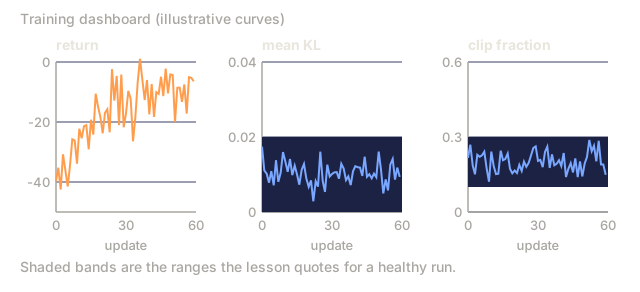
10. Return is noisy, yet mean KL and clip fraction are both in range. What should you check next?Analyze
Three small line charts over 60 updates: a noisy rising return, mean KL hovering between about 0.005 and 0.015 inside a shaded band from 0 to 0.02, and clip fraction between about 0.15 and 0.25 inside a shaded band from 0.1 to 0.3.
Illustrative curves, not a real run.

Pitfalls

  • Clip coefficient mistuned. ε = 0.2 is the de-facto standard. Going to 0.1 makes updates too timid; 0.3+ invites instability.
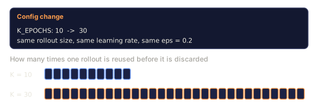
  • Too many epochs. K > 20 routinely destabilizes because the policy drifts far from π_old. Cap epochs, especially for large networks.
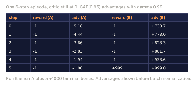
  • No reward normalization. Large reward scales eat into the clip range. Normalize rewards (running std) before computing advantages.
  • Forgetting advantage normalization. Per-batch zero-mean/unit-std normalization is standard. Skipping it wrecks PPO on most benchmarks.
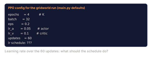
  • Learning rate not decayed. PPO benefits from linear LR decay to zero. Constant LR is often worse.
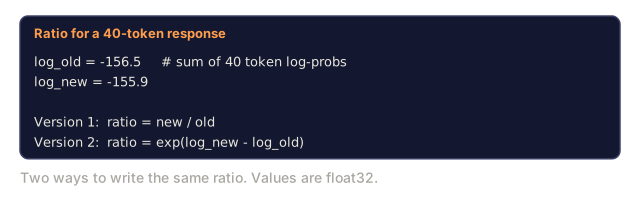
  • Importance ratio math errors. Always exp(log_new - log_old) for numerical stability, not new / old.
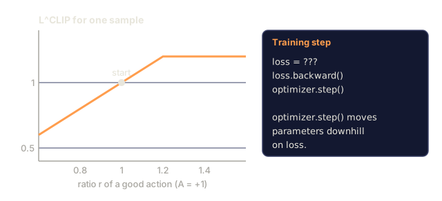
  • Wrong gradient sign. Maximize the surrogate = minimize -L^{CLIP}. A flipped sign is the most common PPO bug.
Check: Pitfalls0/8
1. Why compute the importance ratio as exp(log_new - log_old) rather than new/old?Explain
A card with log_old = -156.5 and log_new = -155.9, the sum of 40 token log-probabilities, and two ways to compute the ratio: new / old and exp(log_new - log_old), with values stored as float32.
Illustrative log-probabilities.
2. The lesson calls a flipped gradient sign the most common PPO bug. What is the correct relationship?Explain
A plot of L^CLIP for one sample with advantage +1 against the ratio, rising until 1.2 and then flat, with a dot at ratio 1, beside a training-step card with loss = ???, loss.backward(), optimizer.step(), noting that the optimizer moves parameters downhill on loss.
3. What does the lesson say about the clip coefficient ε?Explain
Plot of the clipped objective for advantage +1 against the ratio for three clip ranges: eps = 0.1, 0.2 and 0.3, each rising along the diagonal and then flat at 1.1, 1.2 and 1.3 respectively.
Computed from the formula.
4. Why does the lesson warn against skipping reward normalization?Explain
A table for a 6-step gridworld episode: run A gives -1 per step and advantages from about -5 to -1; run B has the same rewards plus a +1000 bonus on the last step and advantages of 731 to 999, shown before normalization.
Computed with the lesson's gae() on a zero critic.
5. What does the lesson recommend for PPO's learning rate schedule?Explain
A config card from the lesson's gridworld code: epochs 4, batch 32, eps 0.2, actor learning rate 0.05, critic learning rate 0.1, 60 updates, and a final line lr schedule: ???.
6. You raise K_EPOCHS from 10 to 30 on the same rollout and training becomes unstable. What is the most likely explanation?Analyze
A config card showing K_EPOCHS changing from 10 to 30 with everything else unchanged, above two rows of small squares, 10 and 30, showing how many passes one rollout gets.
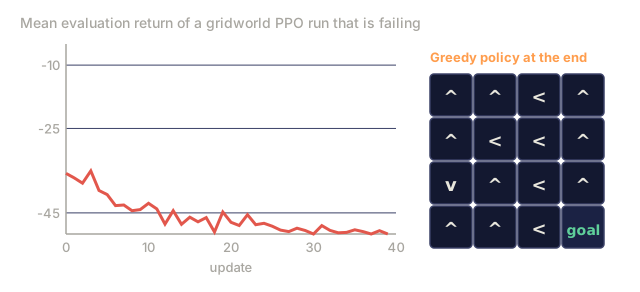
7. Return falls steadily and the policy shifts toward actions with negative advantage. What is the most likely bug?Analyze
Line plot of evaluation return over 40 updates of a gridworld PPO run, falling from -35.6 to -50.0, beside the 4 by 4 greedy policy grid at the end of that run with the goal in the bottom right corner.
Real run of the lesson's gridworld PPO with a small actor step size (0.004) and one change to the update (not shown).
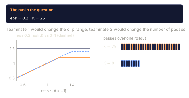
8. A PPO run with ε = 0.2 and K = 25 is unstable. One teammate proposes ε = 0.4 for more room; another proposes cutting K to 8. Which is the better first change?Analyze
The run in the question, eps = 0.2 and K = 25, a plot of the clipped objective for eps 0.2 solid against eps 0.4 dashed, and rows of small squares showing 25 passes against 8 passes over one rollout.

Use It

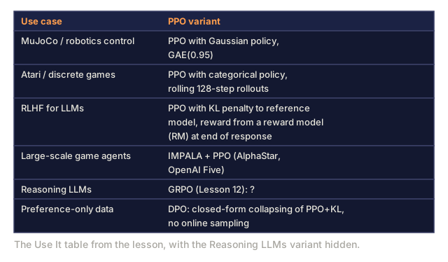
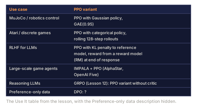
PPO is 2026's default RL algorithm across a surprising number of domains:

Use casePPO variant
MuJoCo / robotics controlPPO with Gaussian policy, GAE(0.95)
Atari / discrete gamesPPO with categorical policy, rolling 128-step rollouts
RLHF for LLMsPPO with KL penalty to reference model, reward from a reward model (RM) at end of response
Large-scale game agentsIMPALA + PPO (AlphaStar, OpenAI Five)
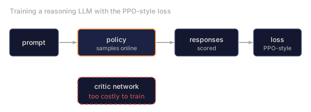
Reasoning LLMsGRPO (Lesson 12): PPO variant without critic
Preference-only dataDPO: closed-form collapsing of PPO+KL, no online sampling

The PPO loss shape (clipped surrogate plus value plus entropy) is the scaffolding for DPO, GRPO, and nearly every RLHF pipeline.
Check: Use It0/5
1. According to the Use It table, how does GRPO relate to PPO for reasoning LLMs?Explain
The lesson's Use It table of six use cases and their PPO variants, with the Reasoning LLMs row showing GRPO (Lesson 12) followed by a question mark in place of its description.
2. How does the Use It table describe DPO's relationship to PPO+KL?Explain
The lesson's Use It table of six use cases and their PPO variants, with the Preference-only data row showing DPO followed by a question mark in place of its description.
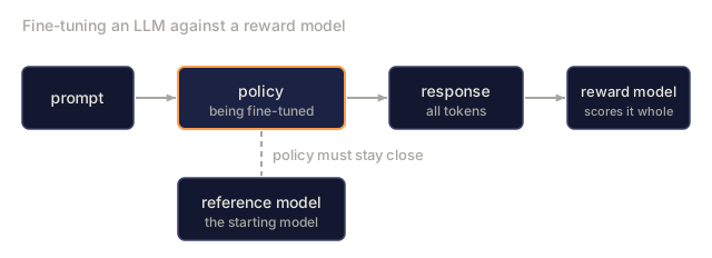
3. You are fine-tuning an LLM with a reward model that scores whole responses, and the policy must stay close to a reference model. Which setup fits?Design
A pipeline: a prompt goes to the policy being fine-tuned, which writes a response, and a reward model scores the whole response; a reference model, the starting model, sits below the policy joined by a dashed line labelled policy must stay close.
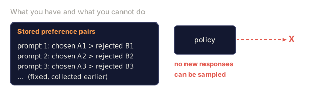
4. Your only data is a fixed set of human preference pairs and you cannot sample from the policy during training. Which approach fits?Design
A card of stored preference pairs, each with a chosen and a rejected response for a prompt, and a policy box with a dashed red arrow crossed out to show that no new responses can be sampled from it during training.
5. You train a reasoning LLM with online sampling and the PPO-style loss, but a critic network is too costly. Which relative of PPO fits?Design
A pipeline: a prompt goes to the policy, which samples responses online; the responses are scored and fed into a PPO-style loss; below the policy a dashed red box labelled critic network, too costly to train.

Ship It

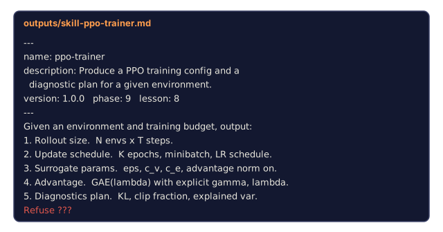
Save as outputs/skill-ppo-trainer.md:

markdown
---
name: ppo-trainer
description: Produce a PPO training config and a diagnostic plan for a given environment.
version: 1.0.0
phase: 9
lesson: 8
tags: [rl, ppo, policy-gradient]
---
 
Given an environment and training budget, output:
 
1. Rollout size. `N` envs × `T` steps.
2. Update schedule. `K` epochs, minibatch size, LR schedule.
3. Surrogate params. `ε` (clip), `c_v`, `c_e`, advantage normalization on.
4. Advantage. GAE(`λ`) with explicit `γ` and `λ`.
5. Diagnostics plan. KL, clip fraction, explained variance thresholds with alerts.
 
Refuse `K > 30` or `ε > 0.3` (unsafe trust region). Refuse any PPO run without advantage normalization or KL/clip monitoring. Flag clip fraction sustained above 0.4 as drift.
Check: Ship It0/1
1. The ppo-trainer skill refuses unsafe configs. Which run does it refuse?Apply
The ppo-trainer skill file from the lesson's Ship It section: front matter with name, description, version, phase 9 and lesson 8, the five output items (rollout size, update schedule, surrogate params, advantage, diagnostics plan), and a final line reading Refuse ??? with the rules hidden.
Author's Note

The first time I broke a PPO run, both my mean KL and clip fraction looked healthy the entire time. The actual bug was reward scale: I'd forgotten to normalize a sparse +1000 terminal bonus, and it was quietly blowing up the value loss while the policy-side diagnostics stayed calm. That's the trap. KL and clip fraction only watch the policy update; they say nothing about the critic. A critic that's diverging in the background can hide behind two healthy-looking numbers for a long time. If your return curve is noisy but KL and clip fraction both check out, look at explained variance next, not just the two diagnostics everyone quotes.

Exercises

  1. Easy. Run PPO on 4×4 GridWorld with ε=0.2, K=4. Compare sample efficiency to A2C (one epoch per rollout) at matched env steps.
  2. Medium. Sweep K ∈ {1, 4, 10, 30}. Plot return vs env steps and track mean KL per update. At what K does KL explode on this task?
  3. Hard. Replace the clipped surrogate with an adaptive KL penalty (β doubled if KL > 2·target, halved if KL < target/2). Compare final return, stability, and clip-free-ness.

Key Terms

TermWhat people sayWhat it actually means
Importance ratio"r_t(θ)"π_θ(a|s) / π_old(a|s); deviation from the policy that collected the data.
Clipped surrogate"PPO's main trick"min(r·A, clip(r, 1-ε, 1+ε)·A); flat gradient past the clip on beneficial side.
Trust region"TRPO / PPO intent"Limit each update's KL to guarantee monotone improvement.
KL penalty"Soft trust region"Alternative PPO: L - β · KL(π_θ || π_old). Adaptive β.
Clip fraction"How often clipping triggers"Diagnostic: should be 0.1-0.3; outside means mistuned.
Multi-epoch training"Data reuse"K epochs on each rollout; variance cost traded for sample efficiency.
On-policy-ish"Mostly on-policy"PPO is nominally on-policy but K>1 epochs uses slightly-off-policy data safely.
PPO-KL"The other PPO"KL-penalty variant; used in RLHF where KL-to-reference is already a constraint.

Further Reading

Code

Ships With