Image Retrieval & Metric Learning
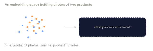
A retrieval system ranks candidates by distance in embedding space. Metric learning is the discipline of shaping that space so the distances actually mean what you want them to.
Learning Objectives
- Explain triplet, contrastive, and proxy-based metric learning losses and pick the right one for a given dataset
- Implement L2-normalisation and cosine similarity correctly and audit the difference between "same item" and "same class" retrieval
- Build a FAISS index, query it by text and by image, and report recall@K for a held-out query set
- Use DINOv2, CLIP, and SigLIP as off-the-shelf embedding backbones and know when each wins
The Problem
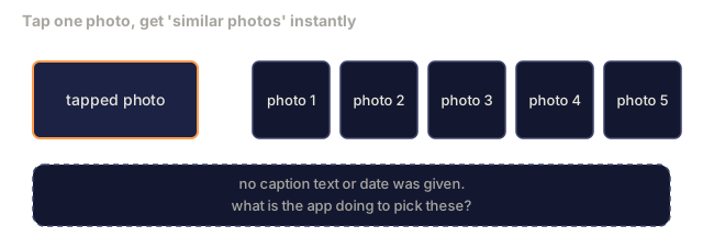
Retrieval is everywhere in production vision: duplicate detection, reverse image search, visual search ("find similar products"), face re-identification, person re-ID for surveillance, instance-level matching for e-commerce. The product question never changes: given this query image, rank my catalogue.
Two design decisions shape the whole system. One is the embedding: what model produces the vectors. The other is the index: how you find nearest neighbours at scale. Both are commodity in 2026 (DINOv2 for the embedding, FAISS for the index), and that commoditization raises the bar instead of lowering it. The hard part is defining what counts as similar for your application, then shaping the embedding space so the distances actually match.
That shaping is metric learning — a small discipline that pays for itself many times over.
The Concept
Retrieval at a glance
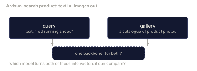
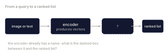
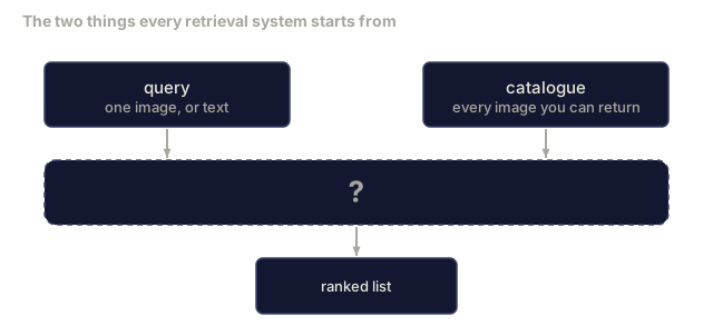
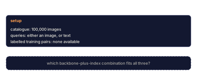
Image retrieval means ranking a gallery of images by similarity to a query, then returning the closest matches first. The query can be an image, or plain text if the encoder maps both into one shared space (CLIP, SigLIP). Every system runs the same shape underneath: encode the query and the catalogue with the same encoder, drop both into a nearest-neighbour index, and rank candidates by distance.

The encoder is the part that changes by model (DINOv2, CLIP, a fine-tune of either). The index is commodity infrastructure: FAISS, covered below. What decides whether the ranked results are actually useful is whether the embedding space puts the right things close together, and that's metric learning's job.
The four loss families
Four loss families cover most of how that space gets shaped:
| Loss | Requires | Pros | Cons |
|---|---|---|---|
| Contrastive | (anchor, positive) + negatives | Simple, works with any pair label | Slow to converge without many negatives |
| Triplet | (anchor, positive, negative) | Intuitive; direct margin control | Hard-triplet mining is expensive |
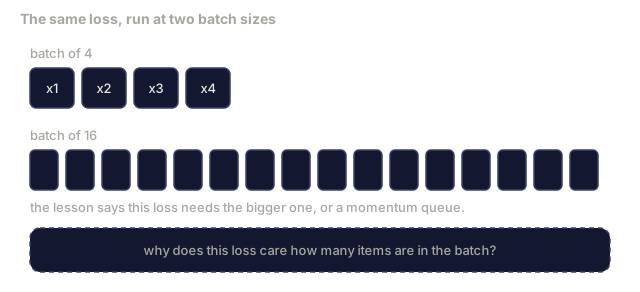
| NT-Xent / InfoNCE | Pairs + batch-mined negatives | Scales to large batches | Needs big batch or momentum queue |
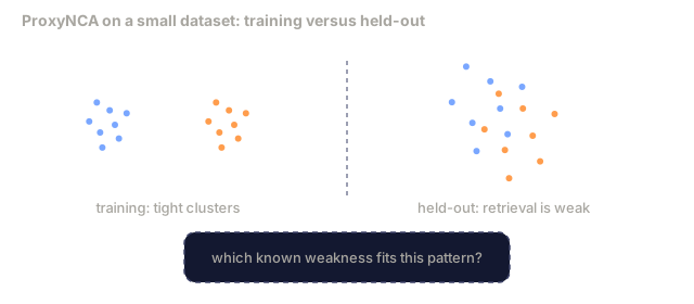
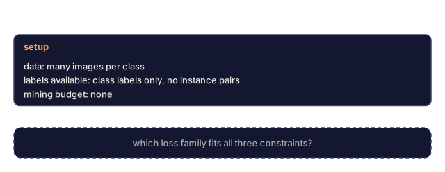
| Proxy-based (ProxyNCA) | Class labels only | Fast, stable, no mining | Can overfit to proxies on small datasets |
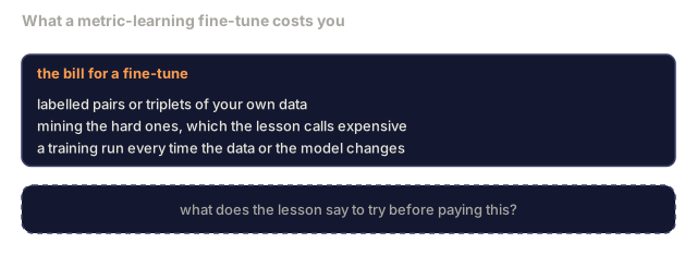
Start with a pretrained backbone for most production use cases, and only reach for a metric-learning fine-tune once the off-the-shelf embeddings underperform on your test set.
Triplet loss formally
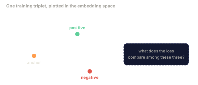
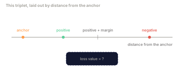
L = max(0, ||f(a) - f(p)||^2 - ||f(a) - f(n)||^2 + margin)
Pull anchor a close to positive p, push it away from negative n, with a margin that keeps a gap between them. The three-image structure generalises to any similarity ordering.
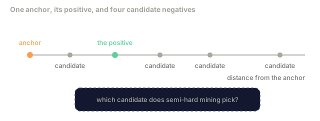
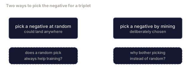
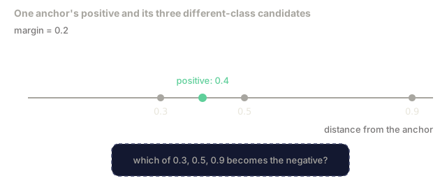
Mining matters: easy triplets (n already far from a) contribute zero loss, so only hard triplets teach the network. Semi-hard mining (n further than p but still within margin) is the 2015 FaceNet recipe, and it still dominates.
Cosine similarity vs L2
Two metrics, two conventions:
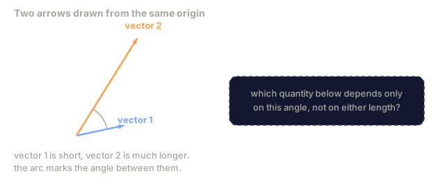
- Cosine: angle between vectors. Requires L2-normalised embeddings.
- L2: Euclidean distance. Works on raw or normalised embeddings, but is usually paired with L2-normalised plus squared L2.
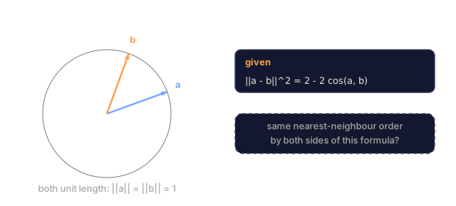
For most modern nets the two are equivalent: ||a - b||^2 = 2 - 2 cos(a, b) when ||a|| = ||b|| = 1. Pick the convention that matches your embedding training. Mixing them silently changes what "nearest" means.
Recall@K
The standard retrieval metric:
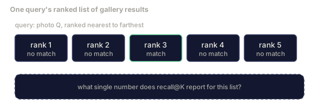
recall@K = fraction of queries where at least one correct match is in the top K results
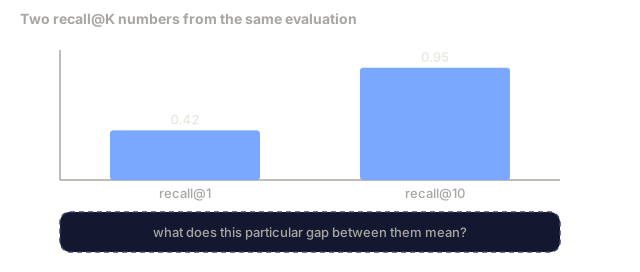
Report recall@1, @5, @10 side by side. A recall@10 above 0.95 with recall@1 below 0.5 means the embedding space has the right structure, but the ranking inside it is noisy. Try longer fine-tunes or a re-ranking step.
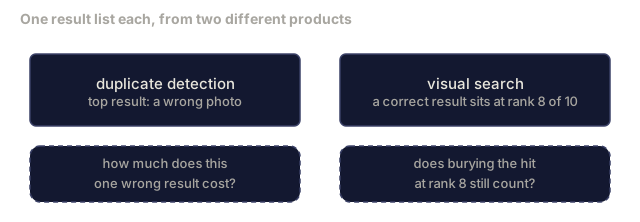
For duplicate detection, precision@K matters more, since every false positive is a user-visible mistake. For visual search, recall@K is the product signal.
FAISS in one paragraph
Facebook AI Similarity Search. The de-facto library for nearest-neighbour search. Three index choices:
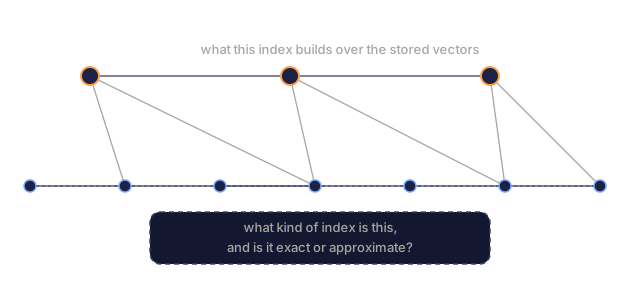
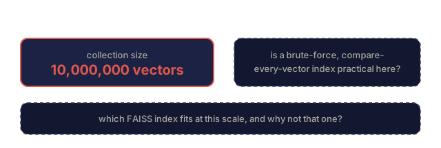
IndexFlatIP/IndexFlatL2: brute force, exact, no training. Use up to ~1M vectors.IndexIVFFlat: partition into K cells, search only the closest few. Approximate, fast, needs training data.IndexHNSW: graph-based, fastest for many queries, at the cost of index size.
For 100k vectors you probably want IndexFlatIP on cosine similarity. For 10M, IndexIVFFlat. Past 100M, add product quantisation (IndexIVFPQ).
Instance-level vs category-level retrieval
Two very different problems with the same name:
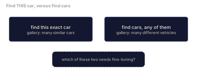
- Category-level: "find cats in my catalogue." Class-conditional similarity; off-the-shelf CLIP / DINOv2 embeddings work well.
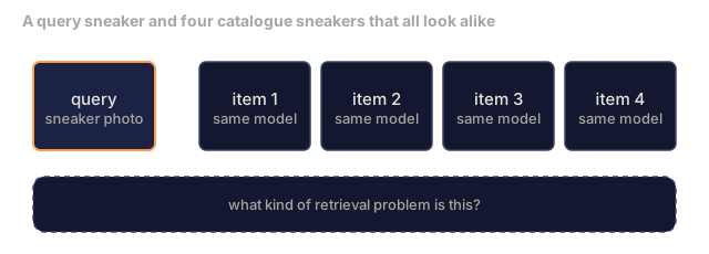
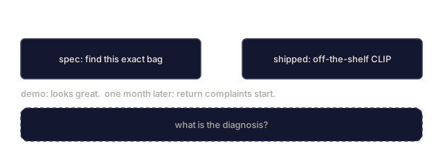
- Instance-level: "find this exact product in my catalogue." Needs fine-grained discrimination between visually similar objects of the same class. Off-the-shelf embeddings underperform here; fine-tuning with metric learning is what closes the gap.
Always ask which one you're actually solving before picking a model.
Build It
Step 1: Triplet loss
import torch
import torch.nn.functional as F

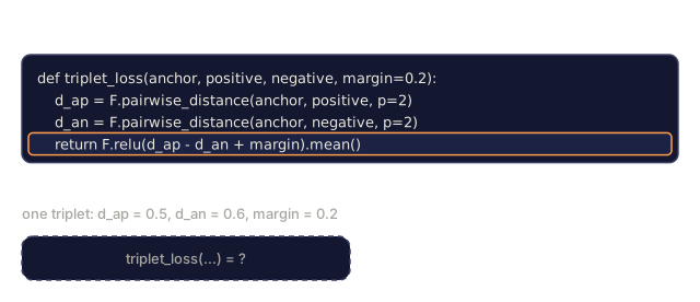
def triplet_loss(anchor, positive, negative, margin=0.2):
    d_ap = F.pairwise_distance(anchor, positive, p=2)
    d_an = F.pairwise_distance(anchor, negative, p=2)
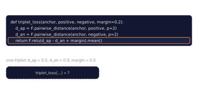
    return F.relu(d_ap - d_an + margin).mean()
One line. Works on L2-normalised or raw embeddings.
Step 2: Semi-hard mining
Given a batch of embeddings and labels, find the hardest semi-hard negative for each anchor.
def semi_hard_negatives(emb, labels, margin=0.2):
    dist = torch.cdist(emb, emb)
    same_class = labels[:, None] == labels[None, :]
    diff_class = ~same_class
    N = emb.size(0)

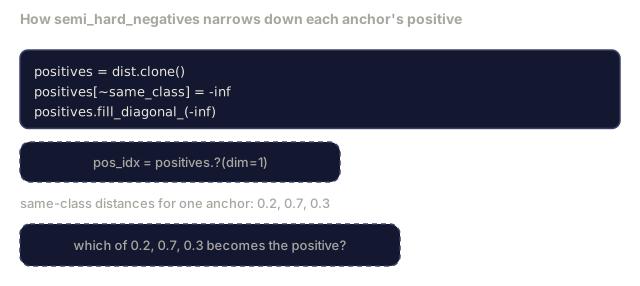
    positives = dist.clone()
    positives[~same_class] = float("-inf")
    positives.fill_diagonal_(float("-inf"))
    pos_idx = positives.argmax(dim=1)

    semi_hard = dist.clone()
    semi_hard[same_class] = float("inf")
    d_ap = dist[torch.arange(N), pos_idx].unsqueeze(1)
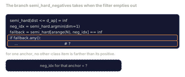
    semi_hard[dist <= d_ap] = float("inf")
    neg_idx = semi_hard.argmin(dim=1)

    fallback_mask = semi_hard[torch.arange(N), neg_idx] == float("inf")
    if fallback_mask.any():
        hardest = dist.clone()
        hardest[same_class] = float("inf")
        neg_idx = torch.where(fallback_mask, hardest.argmin(dim=1), neg_idx)
    return pos_idx, neg_idx
Each anchor gets the hardest positive in-class and a semi-hard negative that is further than the positive but within margin.
Step 3: Recall@K
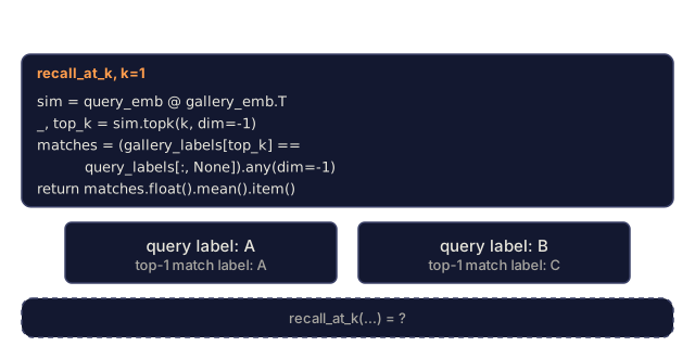
def recall_at_k(query_emb, gallery_emb, query_labels, gallery_labels, k=1):
    sim = query_emb @ gallery_emb.T
    _, top_k = sim.topk(k, dim=-1)
    matches = (gallery_labels[top_k] == query_labels[:, None]).any(dim=-1)
    return matches.float().mean().item()
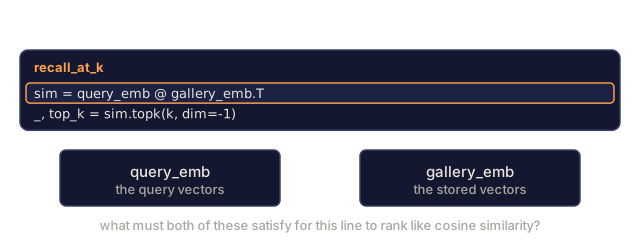
Top-k by inner product on L2-normalised embeddings equals top-k by cosine. Report the mean proportion of queries with at least one correct neighbour.
Step 4: Putting it together
import torch
import torch.nn as nn
from torch.optim import Adam

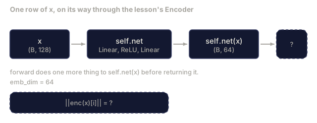
class Encoder(nn.Module):
    def __init__(self, in_dim=128, emb_dim=64):
        super().__init__()
        self.net = nn.Sequential(
            nn.Linear(in_dim, 128), nn.ReLU(),
            nn.Linear(128, emb_dim),
        )

    def forward(self, x):
        return F.normalize(self.net(x), dim=-1)

torch.manual_seed(0)
num_classes = 6
protos = F.normalize(torch.randn(num_classes, 128), dim=-1)

def sample_batch(bs=32):
    labels = torch.randint(0, num_classes, (bs,))
    x = protos[labels] + 0.15 * torch.randn(bs, 128)
    return x, labels

enc = Encoder()
opt = Adam(enc.parameters(), lr=3e-3)

for step in range(200):
    x, y = sample_batch(32)
    emb = enc(x)
    pos_idx, neg_idx = semi_hard_negatives(emb, y)
    loss = triplet_loss(emb, emb[pos_idx], emb[neg_idx])
    opt.zero_grad(); loss.backward(); opt.step()
After a few hundred steps the embedding clusters form one cluster per class.
Use It
Production stacks in 2026:
- DINOv2 + FAISS: general-purpose visual retrieval. Works off-the-shelf.
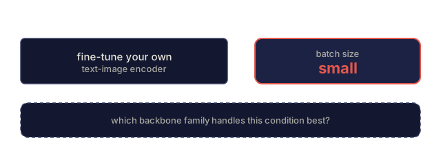
- CLIP or SigLIP + FAISS: for text queries. Off-the-shelf, the two are close in quality; SigLIP's per-pair loss (Lesson 18) makes it the better pick if you fine-tune your own encoder under a small batch size.
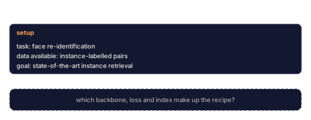
- Fine-tuned DINOv2 + FAISS: instance-level retrieval, face re-ID, fashion, e-commerce.
- Milvus / Weaviate / Qdrant: managed vector DB wrappers around FAISS or HNSW.
For SOTA instance retrieval, the recipe is: DINOv2 backbone, add an embedding head, fine-tune with a triplet or InfoNCE loss on instance-labelled pairs, index in FAISS.
Ship It
This lesson produces:
outputs/prompt-retrieval-loss-picker.md: a prompt that picks triplet / InfoNCE / ProxyNCA for a given retrieval problem.outputs/skill-recall-at-k-runner.md: a skill that writes a clean evaluation harness for recall@K with train/val/gallery splits and proper data contract.
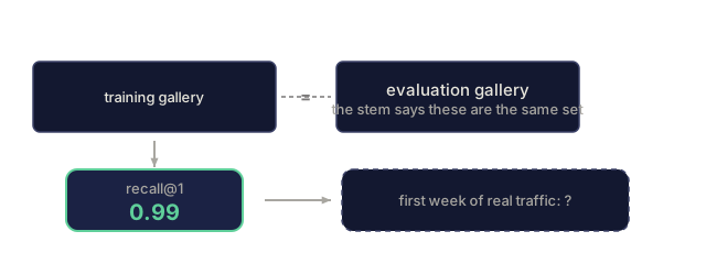
The mistake I see most often here isn't in the loss function, it's in the eval. Someone trains a solid embedding, wires it into FAISS, and reports recall@K against the same gallery the model trained on instead of a genuinely held-out split. Recall@1 comes back at 0.99, everyone's happy — until the model falls apart the first week it sees real traffic, because the real test never ran.
The other trap is conflating instance retrieval with category retrieval. If the spec says "find this exact bag," and you ship a CLIP embedding tuned for "find bags like this," the demo looks great and the return-rate complaints start a month later. Decide which problem you're actually solving before you pick a backbone, not after you've already shipped one.
Exercises
- (Easy) Run the toy example above. Plot the embeddings with PCA before and after training to see the six clusters form.
- (Medium) Add a ProxyNCA loss implementation: one learned "proxy" per class, standard cross-entropy on cosine similarity. Compare convergence speed vs triplet loss on the toy data.
- (Hard) Take 1,000 ImageNet validation images, embed with DINOv2 via HuggingFace, build a FAISS flat index, and report recall@{1, 5, 10} against the same images as queries (should be 1.0) and against a held-out split with ImageNet labels as ground truth.
Key Terms
| Term | What people say | What it actually means |
|---|---|---|
| Metric learning | "Shape the space" | Training an encoder so distances in its output space reflect a target similarity |
| Triplet loss | "Pull and push" | L = max(0, d(a, p) - d(a, n) + margin); the canonical metric-learning loss |
| Semi-hard mining | "Useful negatives" | Negatives further from the anchor than the positive but within margin; empirically the most informative |
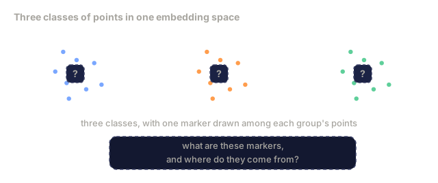
| Proxy-based loss | "Class prototypes" | One learned proxy per class; cross-entropy over similarity-to-proxies; no pair mining |
| Recall@K | "Top-K hit rate" | Fraction of queries with at least one correct result in the top K |
| Instance retrieval | "Find this exact thing" | Fine-grained matching; off-the-shelf features usually underperform |
| FAISS | "The NN library" | Facebook's nearest-neighbour library; supports exact and approximate indexes |
| HNSW | "Graph index" | Hierarchical navigable small world; fast approximate NN, at the cost of a larger index (graph links on top of the vectors) |
Further Reading
- FaceNet: A Unified Embedding for Face Recognition (Schroff et al., 2015): the triplet loss / semi-hard mining paper
- In Defense of the Triplet Loss for Person Re-Identification (Hermans et al., 2017): practical guide to triplet fine-tuning
- FAISS documentation: every index, every trade-off
- SMoT: Metric Learning Taxonomy (Kim et al., 2021): survey of modern losses and their connections
Code
- main.py (python, 94 lines)