The Fourier Transform
Every signal is a sum of sine waves. The Fourier transform tells you which ones, and how strong each one is.
Learning Objectives
- Implement the DFT from scratch and verify it against the O(N log N) Cooley-Tukey FFT
- Interpret frequency coefficients: extract amplitude, phase, and power spectrum from a signal
- Apply the convolution theorem to perform convolution via FFT multiplication
- Connect Fourier frequency decomposition to transformer positional encodings and CNN convolution layers
The Problem
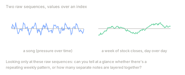
An audio recording is a sequence of pressure measurements over time. A stock price is a sequence of values over days. An image is a grid of pixel intensities over space. All three are data in the time domain (or space domain): you see values changing over some index, and that's it.
Plenty of real patterns don't show up there. Is that audio signal a pure tone or a chord? Does the stock have a weekly cycle? Does the image have a repeating texture? Those are all questions about frequency content, and the time domain simply doesn't show frequency.
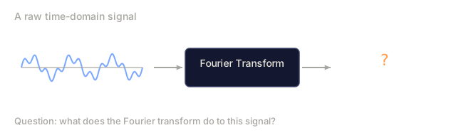
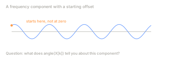
The Fourier transform is the tool that moves data from the time domain into the frequency domain. It decomposes a signal into sine waves of different frequencies, and for each one it hands you an amplitude (how strong it is) and a phase (where it starts).
Frequency-domain thinking shows up constantly in ML. A convolutional layer's convolution operation is multiplication in the frequency domain. Transformer positional encodings represent position through frequency decomposition. Audio models, speech recognition, music generation, run on spectrograms: frequency representations of sound, not waveforms. Time series models hunt for periodic patterns the same way. Learn the Fourier transform once and you have the vocabulary for all of it.
The Concept
The DFT definition
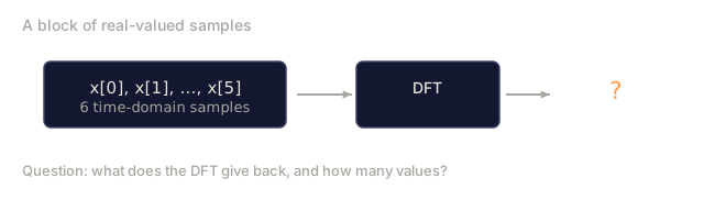
Given N samples x[0], x[1], ..., x[N-1], the Discrete Fourier Transform produces N frequency coefficients X[0], X[1], ..., X[N-1]:
X[k] = sum_{n=0}^{N-1} x[n] * e^(-2*pi*i*k*n/N)

for k = 0, 1, ..., N-1
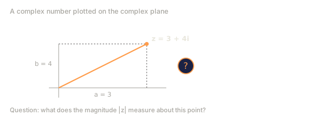
Each X[k] is a complex number: its magnitude |X[k]| gives the amplitude of frequency k, and its phase angle(X[k]) gives that frequency's phase offset.
e^(-2*pi*i*k*n/N) is a rotating phasor at frequency k, and the DFT is really running a correlation: it checks the signal against each of N equally-spaced frequencies in turn. Energy at frequency k makes that correlation large. No energy there and it sits near zero.
What each coefficient means
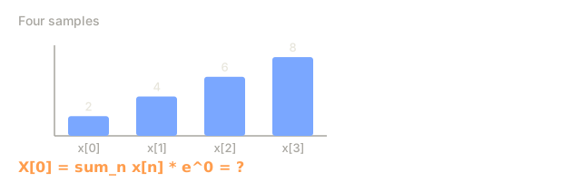
X[0]: the DC component. The sum of all samples, proportional to the mean. It's the constant, zero-frequency offset of the signal.
X[0] = sum_{n=0}^{N-1} x[n] * e^0 = sum of all samples
X[k] for 1 <= k <= N/2: positive frequencies. X[k] represents frequency k cycles per N samples. Higher k means higher frequency: faster oscillation.
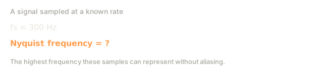
X[N/2]: the Nyquist frequency. The highest frequency you can represent with N samples. Push past it and you get aliasing, high frequencies pretending to be low ones.
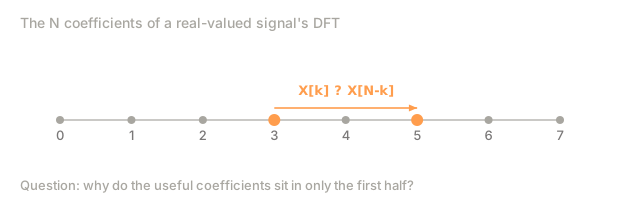
X[k] for N/2 < k < N: negative frequencies. For real-valued signals, X[N-k] = conj(X[k]): the negative frequencies just mirror the positive ones. That's why all the useful information sits in the first N/2 + 1 coefficients.
Inverse DFT
The inverse DFT reconstructs the original signal from its frequency coefficients:
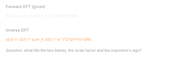
x[n] = (1/N) * sum_{k=0}^{N-1} X[k] * e^(2*pi*i*k*n/N)

for n = 0, 1, ..., N-1
Two things change from the forward DFT: the sign in the exponent flips positive, and a 1/N normalization factor gets added.
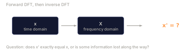
Run the DFT and then the inverse, and you get the exact original signal back: no error, no information lost. The DFT isn't compressing or destroying anything. It's a change of basis, the same information written in a different coordinate system.
The FFT: making it fast
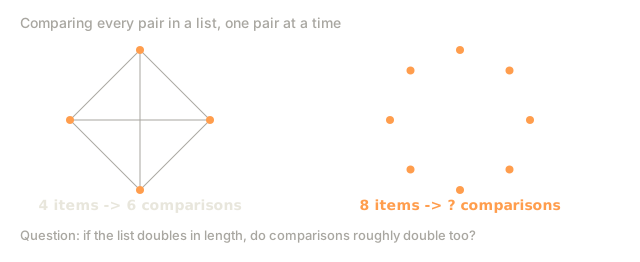
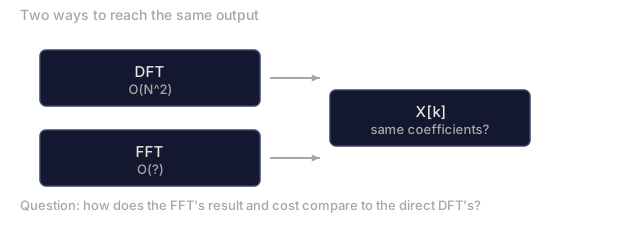
The DFT as defined above is O(N^2): N output coefficients, each one a sum over N input samples. At N = 1 million, that's 10^12 operations.
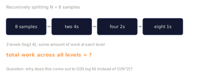
The Fast Fourier Transform computes the identical result in O(N log N): about 20 million operations instead of a trillion, at that same N. That gap is the whole reason frequency analysis is practical at scale.
The Cooley-Tukey algorithm, the most common FFT, gets there by divide and conquer:
- Split the signal into even-indexed and odd-indexed samples.
- Compute the DFT of each half recursively.
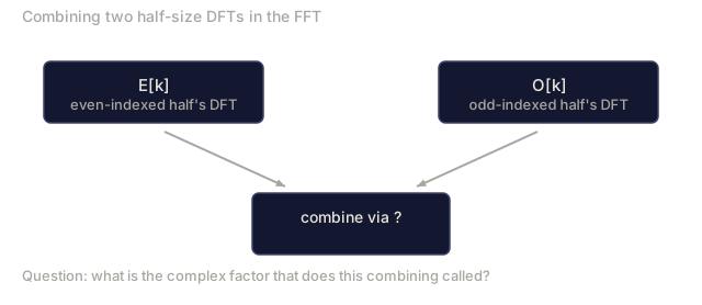
- Combine the two half-size DFTs using "twiddle factors" e^(-2pii*k/N).
X[k] = E[k] + e^(-2*pi*i*k/N) * O[k]          for k = 0, ..., N/2 - 1
X[k + N/2] = E[k] - e^(-2*pi*i*k/N) * O[k]    for k = 0, ..., N/2 - 1

where E = DFT of even-indexed samples
      O = DFT of odd-indexed samples
Each level of recursion does O(N) work, and there are log2(N) levels, so the total comes out to O(N log N).

The catch: the FFT needs the signal length to be a power of 2. In practice, you zero-pad to the next one.
Spectral analysis
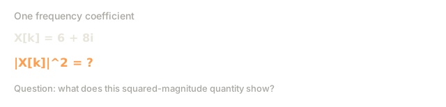
The power spectrum is |X[k]|^2, the squared magnitude of each frequency coefficient. It tells you how much energy sits at each frequency.
The phase spectrum is angle(X[k]), the phase offset of each frequency. Most analysis tasks care only about the power spectrum and throw the phase away.
Power at frequency k:  P[k] = |X[k]|^2 = X[k].real^2 + X[k].imag^2
Phase at frequency k:  phi[k] = atan2(X[k].imag, X[k].real)
Frequency resolution
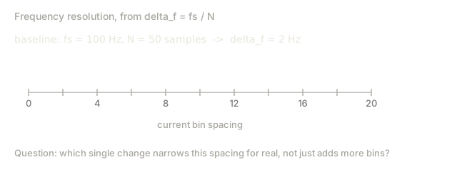
The DFT's frequency resolution comes from two knobs: the number of samples N and the sampling rate fs.
Frequency of bin k:      f_k = k * fs / N
Frequency resolution:    delta_f = fs / N
Maximum frequency:       f_max = fs / 2  (Nyquist)
Want to tell two close frequencies apart? Take more samples. Want to capture higher frequencies at all? Raise the sampling rate.
The convolution theorem
One of the most important results in signal processing, and directly relevant to CNNs.
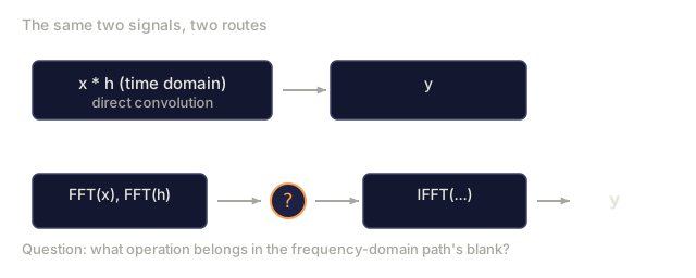
Convolution in the time domain equals pointwise multiplication in the frequency domain.
x * h = IFFT(FFT(x) . FFT(h))

where * is convolution and . is element-wise multiplication
Why it matters:
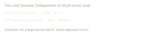
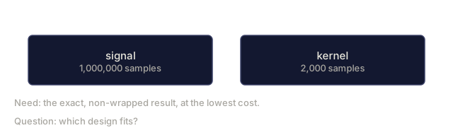
- Direct convolution of two signals of length N and M costs O(N*M).
- FFT-based convolution costs O(N log N): transform both, multiply, transform back.
- For large kernels, that difference is dramatic.
- This is exactly what a convolutional layer with a large receptive field is doing under the hood.
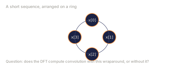
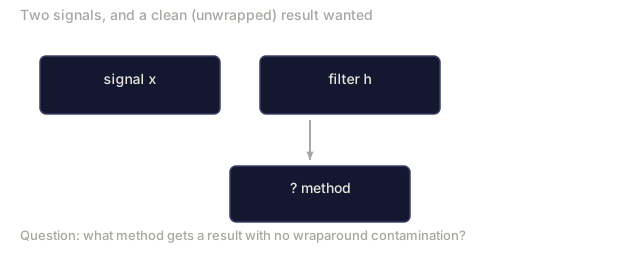
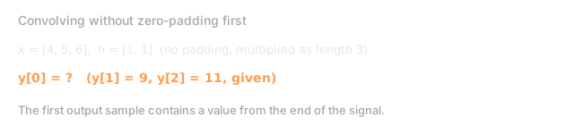
One catch: the DFT computes circular convolution, where the signal wraps around at the edges. For linear convolution (no wraparound), zero-pad both signals to length N + M - 1 first.

Windowing
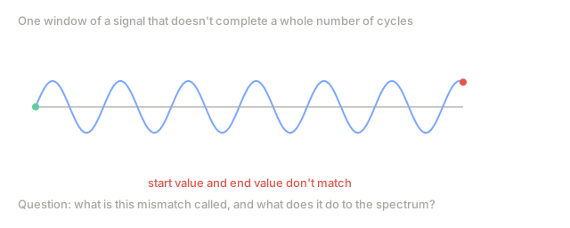
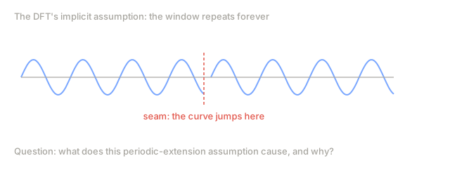
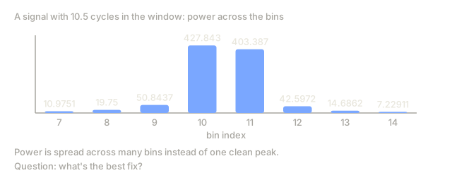
Spectral leakage is spurious high-frequency content that shows up because the DFT assumes the signal is periodic: it treats your N samples as one period of an infinitely repeating signal. If the signal doesn't start and end at the same value, that mismatch creates a discontinuity at the boundary, and the discontinuity leaks into frequencies that were never actually in the signal.
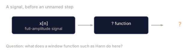
Windowing fixes this by tapering the signal to zero at both ends before you run the DFT.
Common windows:
| Window | Shape | Main lobe width | Side lobe level | Use case |
|---|---|---|---|---|
| Rectangular | Flat (no window) | Narrowest | Highest (-13 dB) | When signal is exactly periodic in N samples |
| Hann | Raised cosine | Moderate | Low (-31 dB) | General purpose spectral analysis |
| Hamming | Modified cosine | Moderate | Lower (-42 dB) | Audio processing, speech analysis |
| Blackman | Triple cosine | Wide | Very low (-58 dB) | When side lobe suppression is critical |
Hann window:    w[n] = 0.5 * (1 - cos(2*pi*n / (N-1)))
Hamming window: w[n] = 0.54 - 0.46 * cos(2*pi*n / (N-1))
Apply a window by multiplying it element-wise with the signal before the DFT: X = DFT(x * w).
DFT properties
| Property | Time Domain | Frequency Domain |
|---|---|---|
| Linearity | ax + by | aX + bY |
| Time shift | x[n - k] | X[f] * e^(-2piifk/N) |
| Frequency shift | x[n] * e^(2piif0n/N) | X[f - f0] |
| Convolution | x * h | X * H (pointwise) |
| Multiplication | x * h (pointwise) | X * H (circular convolution, scaled by 1/N) |
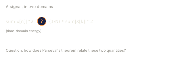
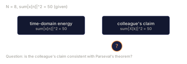
| Parseval's theorem | sum |x[n]|^2 | (1/N) * sum |X[k]|^2 |
| Conjugate symmetry (real input) | x[n] real | X[k] = conj(X[N-k]) |
Two rows there are easy to skim past. Shifting a signal in time only rotates each frequency's phase: the magnitude, how much of that frequency exists, never moves. Shifting a signal's frequency does the mirror-image thing, sliding the whole spectrum over instead. And multiplying two signals pointwise in time turns into a circular convolution in frequency, the flip side of the convolution theorem above.
Parseval's theorem: total energy is the same in both domains. Nothing gets lost or added, only re-expressed.
Connection to positional encodings
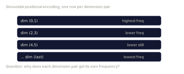
The original Transformer encodes position with sinusoids:
PE(pos, 2i)   = sin(pos / 10000^(2i/d_model))
PE(pos, 2i+1) = cos(pos / 10000^(2i/d_model))
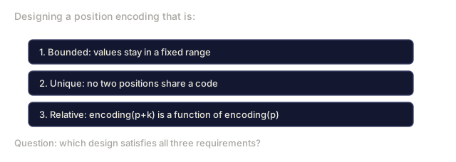
Each dimension pair (2i, 2i+1) oscillates at its own frequency, geometrically spaced from high (dimensions 0, 1) down to low (the last dimensions). Stack them up and every position gets a unique pattern across all frequency bands, the same way a set of Fourier coefficients uniquely pins down a signal.
That construction buys three properties:
- Uniqueness: no two positions share an encoding.
- Bounded values: sin and cos never leave [-1, 1].
- Relative position: the encoding of position p+k is a linear function of the encoding at position p, so the model can learn to attend by relative offset instead of absolute position.
Connection to CNNs
A convolution layer slides a learned filter (kernel) across the input, whether that input is a signal or an image. That sliding operation is, mathematically, convolution.
By the convolution theorem, you could just as well:
- FFT the input
- FFT the kernel
- Multiply the two in the frequency domain
- IFFT the result back
Standard CNNs skip this and use direct convolution, which wins for small 3x3 kernels. But for large kernels or global convolution, FFT-based convolution pulls ahead by a wide margin. Some architectures push this further: FNet replaces attention entirely with an FFT, and gets competitive accuracy at O(N log N) instead of attention's O(N^2).
Spectrograms and the Short-Time Fourier Transform
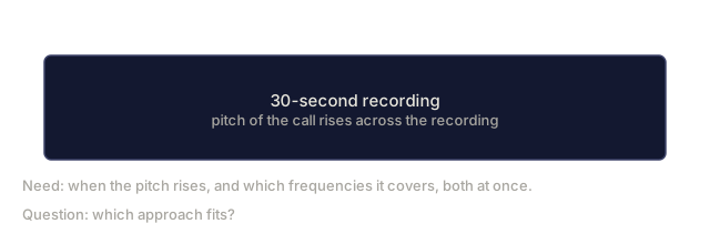
The Short-Time Fourier Transform runs FFTs on overlapping windows of a signal instead of the whole thing at once, then stacks the results into a spectrogram: time on one axis, frequency on the other, and intensity at each point showing how much energy that frequency carried at that moment.
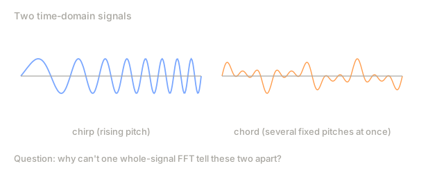
That solves a real gap: a single FFT tells you the frequency content of an entire signal, and nothing about when each frequency happened. A chirp (frequency rising over time) and a chord (every frequency at once) can produce the same magnitude spectrum, even though they sound nothing alike.
STFT procedure:
1. Choose a window size (e.g., 1024 samples)
2. Choose a hop size (e.g., 256 samples -- 75% overlap)
3. For each window position:
   a. Extract the windowed segment
   b. Apply a Hann/Hamming window
   c. Compute FFT
   d. Store the magnitude spectrum as one column of the spectrogram
Spectrograms are the standard input format for audio ML. Speech models like Whisper and DeepSpeech run on mel-spectrograms specifically: the frequency axis gets remapped to the mel scale, which tracks human pitch perception more closely than raw Hz does.
Aliasing
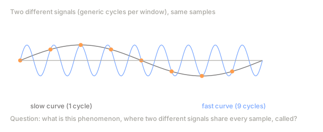
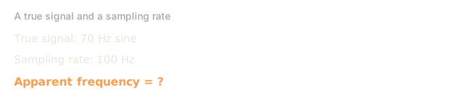
Sample a signal at rate fs and any frequency content above fs/2, the Nyquist frequency, comes back as a fake lower frequency: an aliased copy. A 90 Hz sine wave sampled at 100 Hz produces exactly the same samples as a 10 Hz sine wave. Once you're holding just the samples, there's no way to tell which one you actually recorded.
Example:
  True signal: 90 Hz sine wave
  Sampling rate: 100 Hz
  Apparent frequency: 100 - 90 = 10 Hz

  The samples from the 90 Hz signal at 100 Hz sampling rate
  are identical to the samples from a 10 Hz signal.
  No amount of math can recover the original 90 Hz.
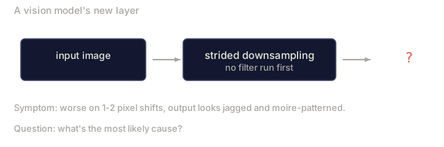
That's why analog-to-digital converters run an anti-aliasing filter first, stripping out anything above Nyquist before sampling happens. The ML version of this shows up when downsampling feature maps without low-pass filtering first. Some architectures fix it with anti-aliased pooling layers.
Zero-padding does not increase resolution
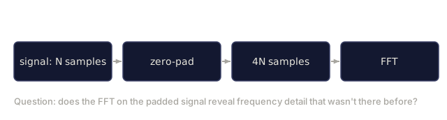
Common misconception: zero-padding a signal before the FFT improves frequency resolution. It doesn't. Zero-padding interpolates between the frequency bins you already have, which makes the spectrum look smoother, but it can't manufacture detail that was never in the original samples.
Real frequency resolution depends only on how long you observed the signal: T = N / fs. Resolving two frequencies separated by delta_f takes at least T = 1 / delta_f seconds of data, full stop. No amount of padding gets around that.



Build It
Step 1: DFT from scratch
The O(N^2) DFT falls straight out of the definition.
import math

class Complex:
    ...

def dft(x):
    N = len(x)
    result = []
    for k in range(N):
        total = Complex(0, 0)
        for n in range(N):
            angle = -2 * math.pi * k * n / N
            w = Complex(math.cos(angle), math.sin(angle))
            xn = x[n] if isinstance(x[n], Complex) else Complex(x[n])
            total = total + xn * w
        result.append(total)
    return result
Step 2: Inverse DFT
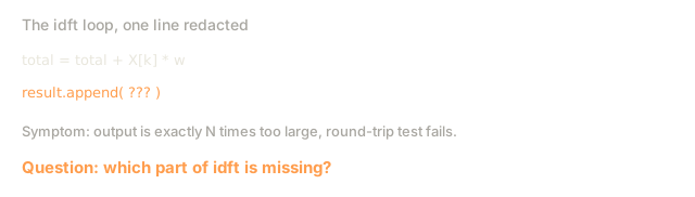
Same structure as the forward DFT: positive exponent, divide by N.
def idft(X):
    N = len(X)
    result = []
    for n in range(N):
        total = Complex(0, 0)
        for k in range(N):
            angle = 2 * math.pi * k * n / N
            w = Complex(math.cos(angle), math.sin(angle))
            total = total + X[k] * w
        result.append(Complex(total.real / N, total.imag / N))
    return result
Step 3: FFT (Cooley-Tukey)
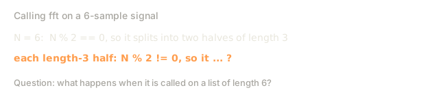
The recursive FFT needs a power-of-2 length: split into even and odd, recurse on each half, combine with twiddle factors.
def fft(x):
    N = len(x)
    if N <= 1:
        return [x[0] if isinstance(x[0], Complex) else Complex(x[0])]
    if N % 2 != 0:
        return dft(x)

    even = fft([x[i] for i in range(0, N, 2)])
    odd = fft([x[i] for i in range(1, N, 2)])

    result = [Complex(0)] * N
    for k in range(N // 2):
        angle = -2 * math.pi * k / N
        twiddle = Complex(math.cos(angle), math.sin(angle))
        t = twiddle * odd[k]
        result[k] = even[k] + t
        result[k + N // 2] = even[k] - t
    return result
Step 4: Spectral analysis helpers
The power-spectrum formula and the convolution theorem from the Concept section turn directly into two small helpers: one squares the magnitude of each coefficient, the other runs convolution through FFT multiplication instead of a nested loop.
def power_spectrum(X):
    return [xk.real ** 2 + xk.imag ** 2 for xk in X]

def convolve_fft(x, h):
    N = len(x) + len(h) - 1
    padded_N = 1
    while padded_N < N:
        padded_N *= 2

    x_padded = x + [0.0] * (padded_N - len(x))
    h_padded = h + [0.0] * (padded_N - len(h))

    X = fft(x_padded)
    H = fft(h_padded)

    Y = [xk * hk for xk, hk in zip(X, H)]

    y = idft(Y)
    return [y[n].real for n in range(N)]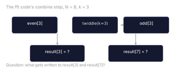


Use It
For real code, reach for numpy's FFT: it's backed by highly optimized C libraries, and there's no reason to hand-roll Cooley-Tukey once you understand it.
import numpy as np

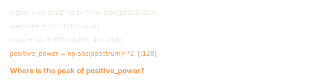
signal = np.sin(2 * np.pi * 5 * np.arange(256) / 256)
spectrum = np.fft.fft(signal)
freqs = np.fft.fftfreq(256, d=1/256)

power = np.abs(spectrum) ** 2

positive_freqs = freqs[:len(freqs)//2]
positive_power = power[:len(power)//2]
For windowing and more advanced spectral analysis:
from scipy.signal import windows, stft

window = windows.hann(256)
windowed = signal * window
spectrum = np.fft.fft(windowed)
For convolution:
from scipy.signal import fftconvolve

result = fftconvolve(signal, kernel, mode='full')
For spectrograms:
from scipy.signal import stft

frequencies, times, Zxx = stft(signal, fs=sample_rate, nperseg=256)
spectrogram = np.abs(Zxx) ** 2
The spectrogram comes out as a matrix of shape (n_frequencies, n_time_frames), where each column is the power spectrum at one time window. That matrix, not the raw waveform, is what audio ML models actually take as input.
Ship It
Run code/fourier.py to generate outputs/prompt-spectral-analyzer.md.
The place this lesson actually pays off isn't when you're writing an FFT by hand. NumPy already did that better than you will, and you should use it. It pays off the day your vision model gets twitchy on small input shifts after you add a strided downsample, and the fix turns out to be exactly the aliasing math above: no anti-aliasing filter, high frequencies folding into low ones, edges coming out jagged and moire-patterned instead of clean. Or you're staring at a spectrogram-based speech model, wondering why the frequency axis looks warped, and the answer is the mel scale from the spectrograms section. Learn the mechanics once here, forget most of the derivations within a year, and you'll still recognize the shape of the problem for the rest of your career.
Exercises
-
Pure tone identification. Create a signal with a single sine wave at an unknown frequency (between 1 and 50 Hz), sampled at 128 Hz for 1 second. Use your DFT to identify the frequency. Verify the answer matches. Now add Gaussian noise with standard deviation 0.5 and repeat. How does noise affect the spectrum?
-
FFT vs DFT verification. Generate a random signal of length 64. Compute both DFT (O(N^2)) and FFT. Verify that all coefficients match to within 1e-10. Time both functions on signals of length 256, 512, 1024, and 2048. Plot the ratio of DFT time to FFT time.
-
Convolution theorem proof by example. Create signal x = [1, 2, 3, 4, 0, 0, 0, 0] and filter h = [1, 1, 1, 0, 0, 0, 0, 0]. Compute their circular convolution directly (nested loop). Then compute it via FFT (transform, multiply, inverse transform). Verify the results match. Now do linear convolution by zero-padding appropriately.
-
Windowing effects. Create a signal that is the sum of two sine waves at 10 Hz and 12 Hz (very close). Sample at 128 Hz for 1 second. Compute the power spectrum with no window, Hann window, and Hamming window. Which window makes it easiest to distinguish the two peaks? Why?
-
Positional encoding analysis. Generate the sinusoidal positional encodings for d_model = 128 and max_pos = 512. For each pair of positions (p1, p2), compute the dot product of their encodings. Show that the dot product depends only on |p1 - p2|, not on the absolute positions. What happens to the dot product as the distance increases?
Key Terms
| Term | What it means |
|---|---|
| DFT (Discrete Fourier Transform) | Converts N time-domain samples into N frequency-domain coefficients. Each coefficient is the correlation with a complex sinusoid at that frequency |
| FFT (Fast Fourier Transform) | An O(N log N) algorithm to compute the DFT. The Cooley-Tukey algorithm splits even/odd indices recursively |
| Inverse DFT | Reconstructs the time-domain signal from frequency coefficients. Same formula as DFT with flipped exponent sign and 1/N scaling |
| Frequency bin | Each index k in the DFT output represents frequency k*fs/N Hz. The "bin" is the discrete frequency slot |
| DC component | X[0], the zero-frequency coefficient. Proportional to the signal mean |
| Nyquist frequency | fs/2, the maximum frequency representable at sampling rate fs. Frequencies above this alias |
| Power spectrum | |X[k]|^2, the squared magnitude of each frequency coefficient. Shows energy distribution across frequencies |
| Phase spectrum | angle(X[k]), the phase offset of each frequency component. Often ignored in analysis |
| Spectral leakage | Spurious frequency content caused by treating a non-periodic signal as periodic. Reduced by windowing |
| Window function | A tapering function (Hann, Hamming, Blackman) applied before DFT to reduce spectral leakage |
| Twiddle factor | The complex exponential e^(-2pii*k/N) used to combine sub-DFTs in the FFT butterfly computation |
| Convolution theorem | Convolution in time domain equals pointwise multiplication in frequency domain. Fundamental to signal processing and CNNs |
| Circular convolution | Convolution where the signal wraps around. This is what the DFT naturally computes |
| Linear convolution | Standard convolution without wraparound. Achieved by zero-padding before DFT |
| Parseval's theorem | Total energy is preserved through the Fourier transform. sum |x[n]|^2 = (1/N) sum |X[k]|^2 |
| Aliasing | When frequencies above Nyquist appear as lower frequencies due to insufficient sampling rate |
Further Reading
- Cooley & Tukey: An Algorithm for the Machine Calculation of Complex Fourier Series (1965) - the original FFT paper that changed computing
- 3Blue1Brown: But what is the Fourier Transform? - the best visual introduction to Fourier transforms
- Lee-Thorp et al.: FNet: Mixing Tokens with Fourier Transforms (2021) - replaces self-attention with FFT in transformers
- Smith: The Scientist and Engineer's Guide to Digital Signal Processing - free online textbook covering FFT, windowing, and spectral analysis in depth
- Vaswani et al.: Attention Is All You Need (2017) - sinusoidal positional encodings derived from Fourier frequency decomposition
- Radford et al.: Whisper (2022) - speech recognition using mel-spectrograms as input representation
Code
- fourier.py (python, 582 lines)