Flow Matching & Rectified Flows
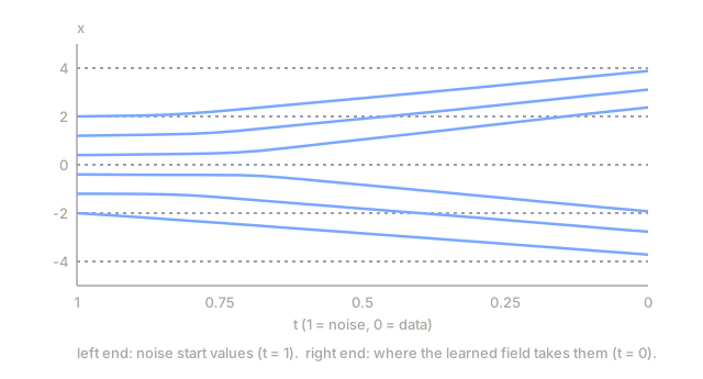
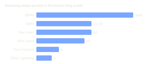
Diffusion samplers take 20-50 steps because they follow a curved path from noise to data. Flow matching (Lipman et al., 2023) and rectified flow (Liu et al., 2022) train toward straight paths instead, and a straighter path needs fewer Euler steps. Stable Diffusion 3, Flux.1, and AudioCraft 2 moved to flow matching in 2024.
Learning Objectives
- Explain why a straight noise-to-data path lets an Euler sampler use far fewer steps than a curved DDPM/DDIM path.
- Derive the conditional flow matching target x_1 - x_0 and write the simulation-free training loss.
- Describe how reflow straightens learned paths and what it costs.
- Implement and compare 1, 2, 4, 8 and 20 step Euler sampling on a 1-D two-mode mixture.
- Choose between flow matching, distillation and both for a given latency target.
The Problem
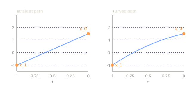
DDPM's reverse process is a 1000-step stochastic walk from N(0, I) back to the data distribution. DDIM collapsed it to 20-50 deterministic steps. You want fewer, ideally one. The blocker is that the ODE behind the reverse process is stiff, because the path it follows is curved.
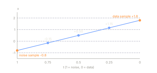
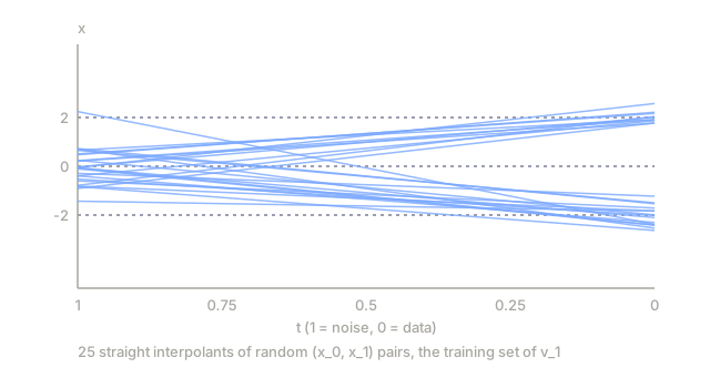
Suppose the path from noise to data were a straight line. Then a single Euler step from t=1 to t=0 would land on the data. Flow matching builds exactly that: define a straight-line interpolation from x_1 ∼ N(0, I) to x_0 ∼ data, train a vector field v_θ(x, t) to match its time derivative, and integrate the field at inference.
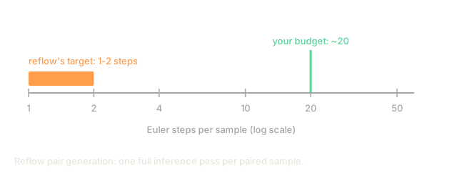
Rectified flow (Liu 2022) goes a step further. A reflow procedure straightens the learned paths iteratively, so each round gives you an ODE closer to linear than the last. After two reflow iterations, a 2-step sampler matches 50-step DDPM quality.
The Concept

Straight-line flow
Define:
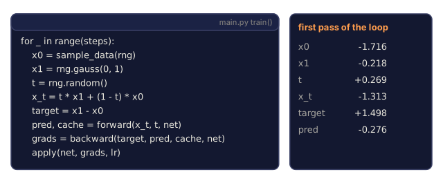
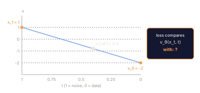
x_t = t · x_1 + (1 - t) · x_0, t ∈ [0, 1]
where x_0 ~ data and x_1 ~ N(0, I). The time derivative along this straight line is constant:
dx_t / dt = x_1 - x_0
Define a neural vector field v_θ(x_t, t) and train it to match this derivative:
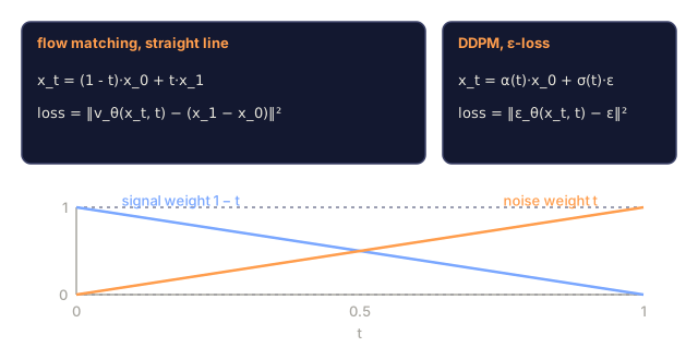
L = E_{x_0, x_1, t} || v_θ(x_t, t) - (x_1 - x_0) ||²
This is the conditional flow matching loss (Lipman 2023). Training is simulation-free: you never unroll the ODE. Just sample (x_0, x_1, t) and regress.
Sampling
At inference, integrate the learned vector field backwards in time:
x_{t-Δt} = x_t - Δt · v_θ(x_t, t)
Start at x_1 ~ N(0, I), Euler-step down to t=0.
Rectified flow (Liu 2022)
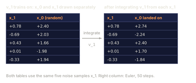
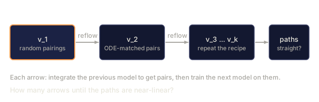
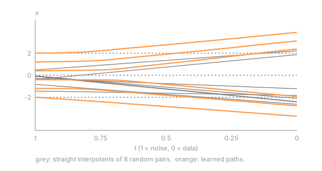
Straight-line flow works, but the learned paths are not actually straight. They curve because many x_0s can map to the same x_1. Rectified flow's reflow step:
- Train flow model v_1 with random pairings.
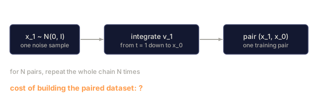
- Sample N pairs
(x_1, x_0)by integrating v_1 fromx_1to its landingx_0. - Train v_2 on those paired examples. Because the pairs are now "ODE-matched", the straight-line interpolant between them is genuinely flatter.
- Repeat.
In practice 2 reflow iterations get you to near-linear, enabling 2-4 step inference. Distilled few-step models like SDXL-Turbo, SD3-Turbo, and LCM attack the same step-count problem from the distillation side.
Why this won for images in 2024
Three reasons made the difference:
- Simulation-free training. You never unroll the ODE during training, so the loss is short to implement.
- Better loss geometry. Straight paths keep the signal-to-noise ratio steadier, while DDPM's ε-loss has poor SNR at the edges of the schedule.
- Faster inference. 4-8 steps at SDXL-Turbo quality, and 1 step with consistency distillation.
Flow matching vs DDPM — the exact connection
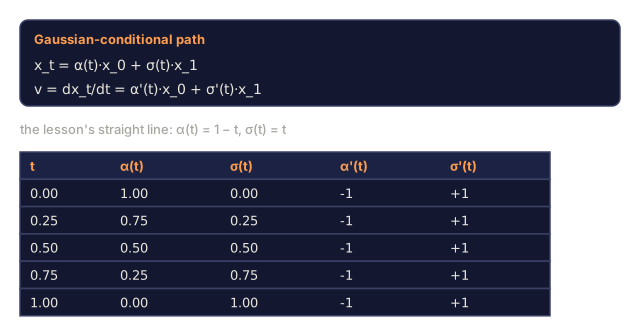
Flow matching with a Gaussian-conditional path is diffusion with a specific noise schedule. Pick the x_t = α(t) x_0 + σ(t) x_1 schedule and flow matching recovers Stratonovich-reformulated diffusion with v = dx_t/dt = α'·x_0 + σ'·x_1. The straight line above is the case α(t) = 1 - t, σ(t) = t, which gives v = -x_0 + x_1 = x_1 - x_0. For Gaussian paths the two are algebraically equivalent.
What flow matching added is a clearer target (a plain velocity), a cleaner loss, and room to experiment with non-Gaussian interpolants.
Build It
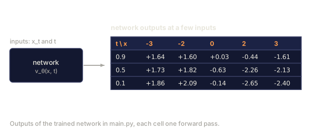
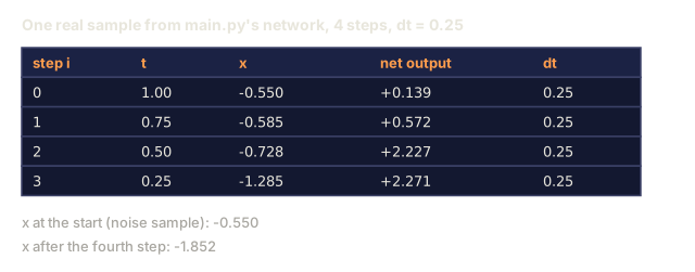
code/main.py implements 1-D flow matching on a two-mode Gaussian mixture. The vector field v_θ(x, t) is a tiny MLP trained with the straight-line target. At inference, integrate 1, 2, 4, 8, and 20 Euler steps and compare sample quality. The snippets below are illustrative; they follow main.py but compress it.
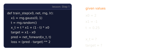
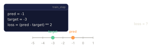
Step 1: training loss
def train_step(x0, net, rng, lr):
    x1 = rng.gauss(0, 1)
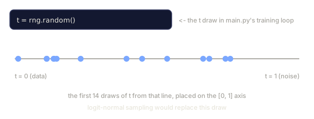
    t = rng.random()
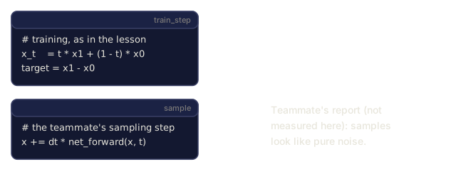
    x_t = t * x1 + (1 - t) * x0
    target = x1 - x0
    pred = net_forward(x_t, t)
    loss = (pred - target) ** 2
    # backprop + update
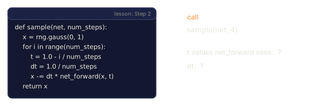
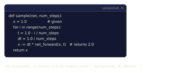
Step 2: multi-step inference
def sample(net, num_steps):
    x = rng.gauss(0, 1)
    for i in range(num_steps):
        t = 1.0 - i / num_steps
        dt = 1.0 / num_steps
        x -= dt * net_forward(x, t)
    return x
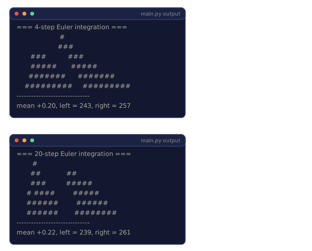
Step 3: compare step counts
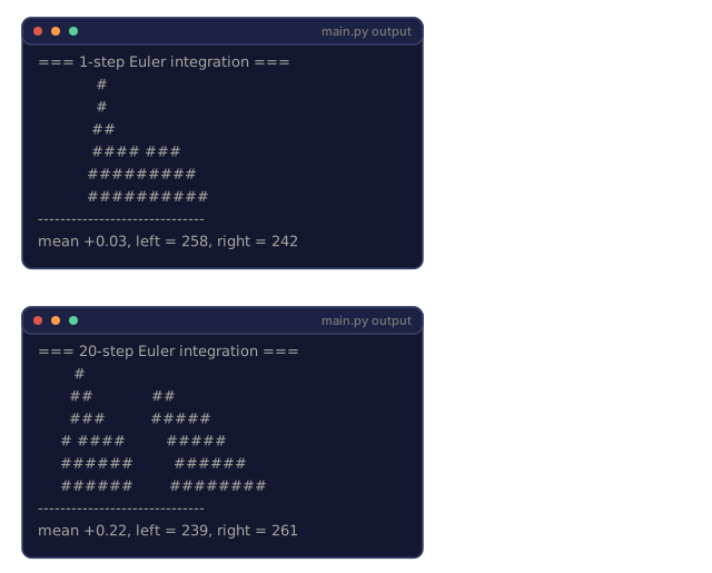
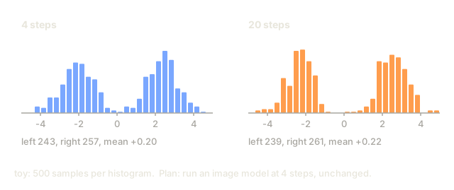
main.py prints a histogram for each step count, plus the sample mean and how many samples landed on each side of zero. Compare the 4-step and 20-step histograms by eye. If they look alike, you have cut the sampling cost by 5x for this toy, and latency scales with step count in a real model too.
Pitfalls
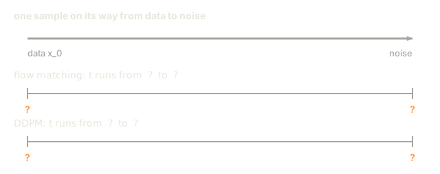
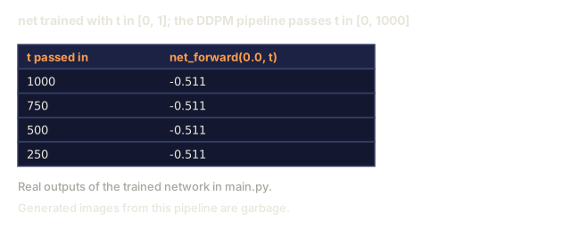
- Time parameterization. Flow matching uses
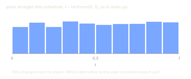
t ∈ [0, 1]witht=0at data,t=1at noise. DDPM usest ∈ [0, T]witht=0at data,t=Tat noise. Same direction, different scale. Papers get this wrong constantly. - Schedule choice. Rectified flow's straight line is the standard flow-matching schedule, but you can use cosine or logit-normal t-sampling (SD3 does this) for better scale coverage.
- Reflow cost. Generating the paired dataset for reflow is a full inference pass per sample. Only do reflow when you really need 1-2 step inference.
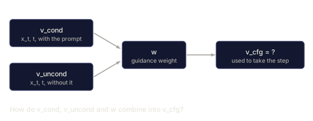
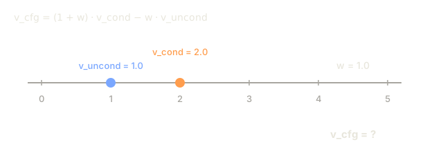
- Classifier-free guidance still applies. Swap ε for v in the linear combination:
v_cfg = (1+w) v_cond - w v_uncond.
Use It
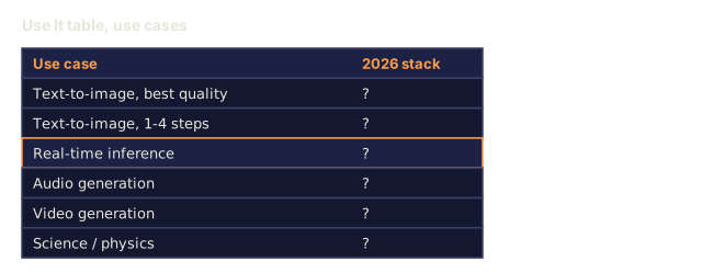
| Use case | 2026 stack |
|---|---|
| Text-to-image, best quality | Flow matching: SD3, Flux.1-dev |
| Text-to-image, 1-4 steps | Distilled flow matching: Flux.1-schnell, SD3-Turbo, SDXL-Turbo |
| Real-time inference | Consistency distillation from a flow-matched base (LCM, PCM) |
| Audio generation | Flow matching: Stable Audio 2.5, AudioCraft 2 |
| Video generation | Flow matching mixed with diffusion (Sora, Veo, Stable Video) |
| Science / physics (particle trajectories, molecules) | Flow matching + equivariant vector field |
Whenever a paper says "faster than diffusion" in 2025-2026, it is almost always flow matching + distillation.
Ship It
Save outputs/skill-fm-tuner.md. Skill takes a diffusion-style model spec and converts it to a flow-matching training config: schedule choice, time sampling distribution (uniform / logit-normal), optimizer, reflow plan, target step count, eval protocol.
I'd run main.py before rereading the derivation. It trains a tiny MLP on a 1-D two-mode mixture with the straight-line target, then samples with 1, 2, 4, 8, and 20 Euler steps. Each run prints a histogram, the sample mean, and a count of samples on each side of zero. The backward pass is hand-written, so nothing sits between you and the regression.
The part I'd reread until it feels boring is the training step. x_t is t * x1 + (1 - t) * x0, the target is x1 - x0, and the loss is a squared error between the net's output and that target. The ODE never gets unrolled during training, which is the whole meaning of simulation-free here.
I'd also read the step-count comparison with some skepticism. The toy is one-dimensional with two tight modes, and the net sees t through a few extra input features (t, t², and a sine and cosine). So the 1-step result, a single blob near zero between the two modes with samples split about evenly across zero, says little about image models. Check the histogram, not just the left/right counts. The closing print statement in main.py compares against DDPM, but the script never runs a DDPM, so treat that line as a hint to test yourself. The reflow exercise is where the straightening claim gets tested properly.
Exercises
- Easy. Run
code/main.pyand compare the 1-step and 20-step histograms against the true two-mode distribution. - Medium. Switch from uniform
tsampling to logit-normal (concentrates sampling at mid-t). Does the model quality improve? - Hard. Implement one reflow iteration: generate paired (x_0, x_1) by integrating the first model, train a second model on the pairs, and compare 1-step sample quality.
Key Terms
| Term | What people say | What it actually means |
|---|---|---|
| Flow matching | "Straight-line diffusion" | Train v_θ(x, t) to match x_1 - x_0 along an interpolant. |
| Rectified flow | "Reflow" | Iterative procedure that straightens learned flows. |
| Velocity field | "v_θ" | Output of the model, the direction to move x_t. |
| Straight-line interpolant | "The path" | x_t = (1-t)·x_0 + t·x_1; trivial target derivative. |
| Euler sampler | "1st order ODE solver" | Simplest integrator; works well when paths are straight. |
| Logit-normal t | "SD3 sampling" | Concentrate t sampling toward mid-values where gradients are strongest. |
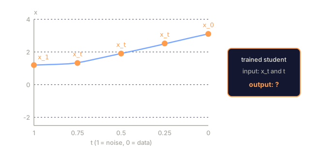
| Consistency distillation | "1-step sampler" | Train a student to map any x_t directly to x_0. |
| CFG with velocity | "v-CFG" | v_cfg = (1+w) v_cond - w v_uncond; same trick, new variable. |
Production note: Flux.1-schnell is flow matching at its fastest
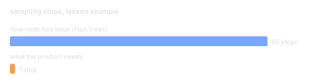
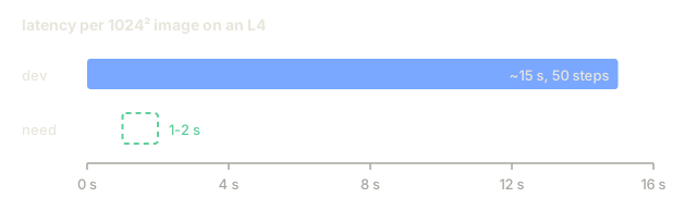
Flux.1-schnell is the clearest production example: a flow-matched DiT distilled to 1-4 inference steps while keeping Flux-dev-grade quality. Niels' "Run Flux on an 8GB machine" notebook is the reference deployment recipe: T5 + CLIP encode, quantized MMDiT denoise (in 4 steps for schnell vs 50 for dev), VAE decode. The cost accounting:
| Variant | Steps | Latency at 1024² on L4 | Total FLOPs (relative) |
|---|---|---|---|
| Flux.1-dev (raw) | 50 | ~15 s | 1.0× |
| Flux.1-schnell | 4 | ~1.2 s | 0.08× (12× faster) |
| SDXL-base | 30 | ~4 s | 0.25× |
| SDXL-Lightning 2-step | 2 | ~0.3 s | 0.03× |
The production rule: a flow-matched base plus distillation is the 2026 default for fast text-to-image. Every major vendor ships this combo: SD3-Turbo (SD3 + flow + distillation), Flux-schnell (Flux-dev + rectified-flow straightening), CogView-4-Flash. Pure diffusion bases exist only for legacy checkpoints.
Further Reading
- Liu, Gong, Liu (2022). Flow Straight and Fast: Learning to Generate and Transfer Data with Rectified Flow: rectified flow.
- Lipman et al. (2023). Flow Matching for Generative Modeling: flow matching.
- Esser et al. (2024). Scaling Rectified Flow Transformers for High-Resolution Image Synthesis: SD3, rectified flow at scale.
- Albergo, Vanden-Eijnden (2023). Stochastic Interpolants: general framework that covers FM + diffusion.
- Song et al. (2023). Consistency Models: 1-step distillation of diffusion / flow.
- Sauer et al. (2023). Adversarial Diffusion Distillation (SDXL-Turbo): turbo variant.
- Black Forest Labs (2024). Flux.1 models: flow matching in production.
Code
- main.py (python, 149 lines)