TAI BUI
Back to curriculum
BuildPython

3D Generation

3D has the most to gain from 2D models, because photos are plentiful and 3D data is not. The 2023 breakthrough was 3D Gaussian Splatting. The 2024-2026 push puts multi-view diffusion and 3D reconstruction on top of it, so one prompt or one photo can produce an object or a scene.

TIME: ~45 minutesPREREQUISITES: Phase 4 (Vision), Phase 8 · 07 (Latent Diffusion)

Learning Objectives

  • Explain why 3D generation is hard (representation, data scarcity, memory, supervision) and how the 2026 stack splits it into multi-view diffusion plus 3D reconstruction.
  • Describe 3D Gaussian Splatting, including the parameters each Gaussian carries and why a differentiable renderer lets you fit it by gradient descent.
  • Compare NeRF, Gaussian splatting, SDS-based text-to-3D, and direct image-to-3D models by speed and output type.
  • Build a toy 2D splat fit and explain how finite differences stand in for a differentiable renderer.
  • Pick a pipeline for a 3D brief and name the pitfalls that follow: view inconsistency, back-side hallucination, splat explosion, and topology.

The Problem

3D content is painful for four reasons:

  • Representation. Meshes, point clouds, voxel grids, signed distance fields (SDFs), neural radiance fields (NeRFs), 3D Gaussians. Each one trades something away.
  • Data scarcity. ImageNet has 14M images. The largest clean 3D dataset (Objaverse-XL, 2023) has ~10M objects, and most are low quality.
  • Memory. A 512³ voxel grid is 128M voxels, and a useful scene NeRF needs 1M samples/ray. Generating is harder than reconstructing.
  • Supervision. A 2D image gives you the pixels. For 3D you usually get a handful of 2D views and have to lift them into 3D yourself.

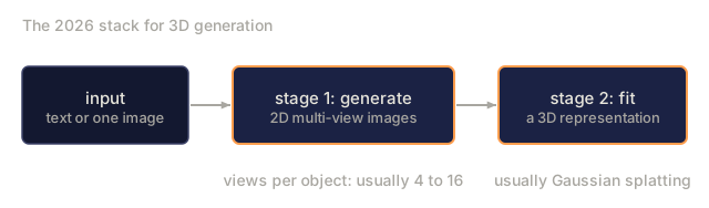
The 2026 stack splits the problem in two. First, generate 2D multi-view images with a diffusion model. Second, fit a 3D representation (usually Gaussian splatting) to those images.
Warm-up0/3
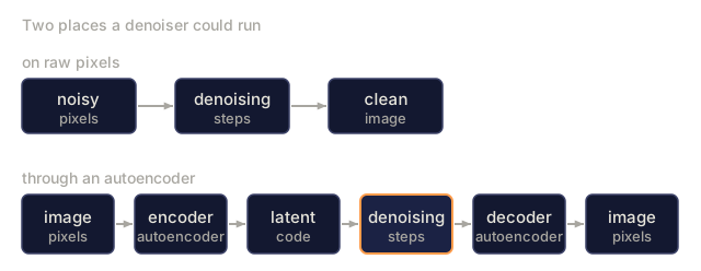
1. Why does latent diffusion run its denoising steps on an autoencoder's latent code instead of on raw pixels?Warm-up
Two flow diagrams. The first runs denoising steps directly on noisy pixels to get a clean image. The second sends an image through an autoencoder encoder to a latent code, runs denoising steps, and decodes back to an image.
Schematic of the two setups the question compares.
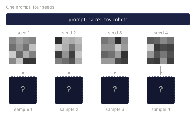
2. You sample four images from a text-to-image diffusion model with one prompt, "a red toy robot", and four different seeds. What do you expect?Warm-up
A prompt box reading "a red toy robot" above four columns. Each column starts from its own random-noise tile labelled seed 1 to 4, with an arrow down to an empty dashed box for sample 1 to 4 marked with a question mark.
Noise tiles are random numbers drawn for illustration, not real model inputs.
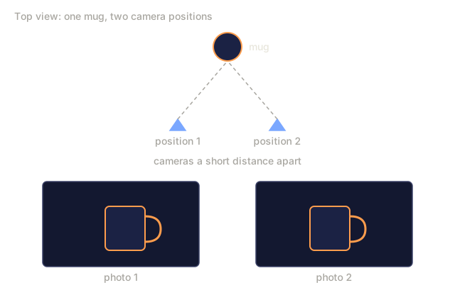
3. You photograph a mug from two slightly different positions. What can the pair of photos give you that a single photo cannot?Warm-up
A top-down sketch of a mug with two cameras a short distance apart, and below it two photo frames, one from each camera, each showing the mug seen from the side with its handle.
Schematic. Camera spacing and the small sideways offset of the mug between the two photos are illustrative.
Check: The Problem0/2
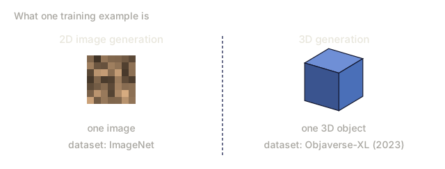
1. Why is training data a bigger obstacle for 3D generation than for 2D image generation?Explain
Two columns. Under 2D image generation, a small pixel grid labelled one image from the ImageNet dataset. Under 3D generation, a cube labelled one 3D object from the Objaverse-XL (2023) dataset.
Pictograms only; no sizes shown.
2. Why does the 2026 stack generate multi-view images first and fit a 3D representation afterward?Explain
A three-box flow: input of text or one image, then stage 1 generating 2D multi-view images, then stage 2 fitting a 3D representation. Notes say usually 4 to 16 views per object and usually Gaussian splatting.
From the lesson's Problem and Concept sections.

The Concept

3D generation: multi-view diffusion + 3D reconstruction

Representation: 3D Gaussian Splatting (Kerbl et al., 2023)

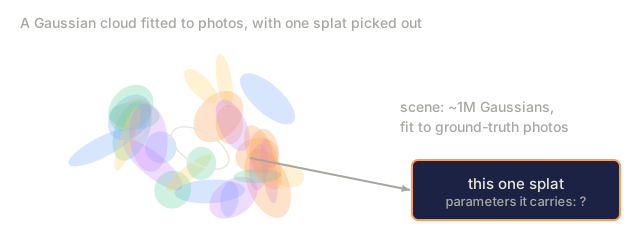
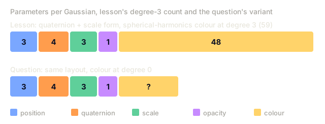
A scene becomes a cloud of ~1M 3D Gaussians. Each has 59 parameters: position (3), covariance (6, or quaternion 4 + scale 3), opacity (1), spherical-harmonics color (48 at degree 3, 3 at degree 0).

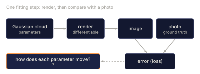
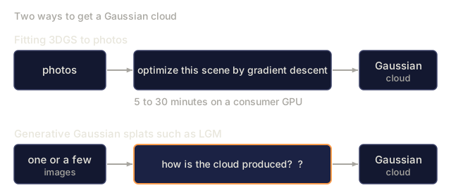
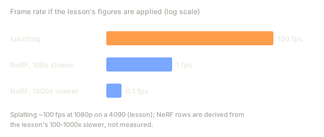
Rendering is projection plus alpha-compositing. It is fast (~100 fps at 1080p on a 4090) and differentiable, so you fit it by gradient descent against ground-truth photos. A scene fits in 5-30 minutes on a consumer GPU.

Two 2023-2024 ideas build on this:

  • Generative Gaussian splats. LGM predicts a Gaussian cloud directly from a few images. LRM and InstantMesh use the same feed-forward idea but output a triplane and a mesh instead (see the table below).
  • 4D Gaussian Splatting. Gaussians with per-frame offsets, for dynamic scenes.

Multi-view diffusion

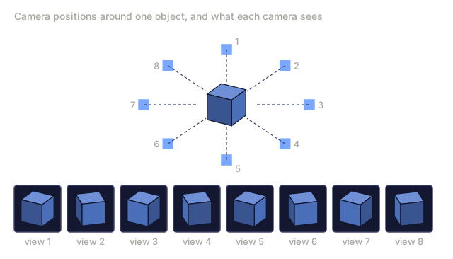
Fine-tune a pretrained image diffusion model so it generates several consistent views of one object from a text prompt or a single image. Examples: Zero123 (Liu et al., 2023), MVDream (Shi et al., 2023), SV3D (Stability, 2024), CAT3D (Google, 2024). These usually output 4-16 views around the object, which you lift to 3D with Gaussian splatting or a NeRF.

Text-to-3D pipelines

ModelInputOutputTime
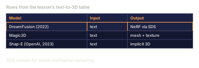
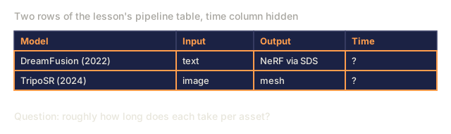
DreamFusion (2022)textNeRF via SDS~1 hour per asset
Magic3Dtextmesh + texture~40 min
Shap-E (OpenAI, 2023)textimplicit 3D~1 min
SJC / ProlificDreamertextNeRF / mesh~30 min
LRM (Meta, 2023)imagetriplane~5 s
InstantMesh (2024)imagemesh~10 s
SV3D (Stability, 2024)imagenovel views~2 min
CAT3D (Google, 2024)1-64 images3D NeRF~1 min
TripoSR (2024)imagemesh~1 s
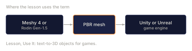
Meshy 4 (2025)text + imagePBR mesh~30 s
Rodin Gen-1.5 (2025)text + imagePBR mesh~60 s
Tencent Hunyuan3D 2.0 (2025)imagemesh~30 s

The 2025-2026 direction is direct text-to-mesh models with PBR materials that game engines can use. For general objects, the multi-view diffusion intermediate step remains the best-performing recipe.

NeRF (for context)

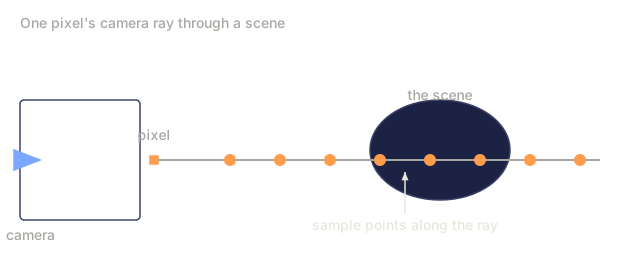
Neural Radiance Field (Mildenhall et al., 2020). A tiny MLP takes (x, y, z, view direction) and outputs (color, density), and you render by integrating along rays. Quality beats mesh-based novel-view synthesis, but rendering is 100-1000x slower. Gaussian splatting has replaced it for most real-time use, though NeRF still dominates research.
Check: The Concept0/12
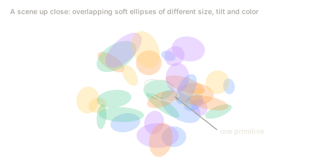
1. What is 3D Gaussian Splatting?Define
A cluster of about thirty overlapping translucent ellipses in several colors, with different sizes and tilts, one of them outlined and labelled one primitive.
Illustrative: ellipses are drawn at random, not taken from a real scene.
2. What is a NeRF (neural radiance field)?Define
A camera on the left sends one ray through a pixel into a scene shown as an oval. Eight dots are marked along the ray, labelled sample points.
Schematic of a neural radiance field rendering one pixel. The number of sample points is illustrative.
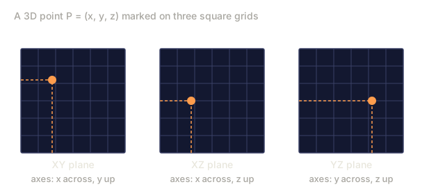
3. What is a triplane representation?Define
Three square grids labelled XY plane, XZ plane and YZ plane, each with one orange dot showing where a single 3D point P lands on that plane, with dashed guide lines to the axes.
Schematic with an illustrative point, P = (0.3, 0.7, 0.5).
4. What is score distillation sampling (SDS)?Define
Three rows of the lesson's text-to-3D table with model, input and output columns: DreamFusion text to NeRF via SDS (highlighted), Magic3D text to mesh plus texture, Shap-E text to implicit 3D. A line expands SDS as score distillation sampling.
Rows copied from the lesson, time column left out.
5. What is multi-view diffusion?Define
A top-down ring of eight numbered camera positions around a small cube, and below it eight thumbnail tiles, view 1 to view 8, each showing the cube from the matching angle.
Illustrative: 8 positions (the lesson says these models usually output 4 to 16 views). Cube views are rendered by the script.
6. Which set of per-Gaussian parameters does 3D Gaussian Splatting fit?Explain
A cloud of overlapping translucent ellipses with one outlined, and an arrow from it to a box reading this one splat, parameters it carries: question mark. Notes say about one million Gaussians per scene, fit against ground-truth photos.
Illustrative cloud drawn at random; the one-million figure is from the lesson.
7. Why does a differentiable renderer let you fit a Gaussian cloud by gradient descent?Explain
A flow diagram: a Gaussian cloud's parameters go through a differentiable render to an image, which is compared with a ground-truth photo to give an error. A dashed arrow from the error points to a highlighted box asking how each parameter moves, with a question mark.
Schematic of one fitting step.
8. How does a generative Gaussian splat model such as LGM differ from fitting 3DGS to photos?Explain
Two rows ending in a Gaussian cloud. Row one: photos, then optimize this scene by gradient descent taking 5 to 30 minutes on a consumer GPU. Row two: one or a few images, then a highlighted box asking how the cloud is produced, with a question mark.
Fit time is the lesson's figure for fitting a scene.
9. In the pipeline table, roughly how long does DreamFusion take per asset compared with TripoSR?Explain
A table with columns model, input, output and time. DreamFusion (2022), text to NeRF via SDS, and TripoSR (2024), image to mesh, are listed with the time column showing question marks.
Rows copied from the lesson's pipeline table, times hidden.
10. Why is NeRF rendering 100-1000x slower than Gaussian splatting?Explain
Three horizontal bars on a log scale of frames per second: splatting at 100, NeRF at 100 times slower giving 1, and NeRF at 1000 times slower giving 0.1.
Splatting fps is the lesson's figure; the NeRF bars are derived from its 100-1000x range.
11. Using the quaternion-plus-scale form of covariance and degree-0 spherical-harmonics color, how many parameters does one Gaussian carry?Apply
Two segmented bars. The first shows the lesson's degree-3 layout: position 3, quaternion 4, scale 3, opacity 1, colour 48, totalling 59. The second repeats position, quaternion, scale and opacity and shows a question mark for the degree-0 colour block.
Counts from the lesson's Concept section; bar widths are not to scale.
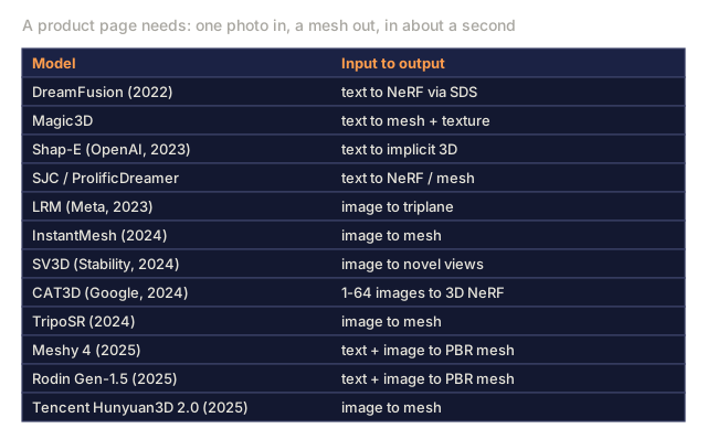
12. A product page needs a mesh from one photo in about a second. Which model in the pipeline table fits?Apply
The lesson's pipeline table of twelve models with model, input and output columns, under a heading stating the need: one photo in, a mesh out, in about a second. The time column is left out.
Rows copied from the lesson's pipeline table, time column hidden.

Build It

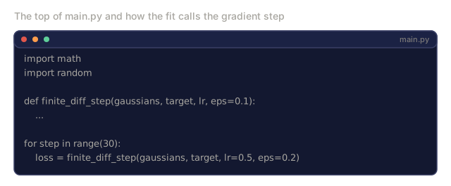
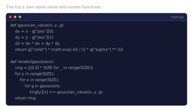
code/main.py is a toy 2D "Gaussian splatting" fit. The target is a 12x12 image with a bright blob in the upper-left and a dimmer one in the lower-right. Each splat has a position, a single sigma (so it is round, not a full covariance), and a color, and the render is the sum of all splats. The fit nudges those parameters to cut the MSE against the target. That gives you the two core operations: forward render and fit. One difference from the snippets below: main.py gets its gradients by finite differences (nudge a parameter by eps, re-render, compare the loss), because there is no autograd in it. Real 3DGS gets exact gradients through the differentiable renderer.

Step 1: 2D Gaussian splat

python
def gaussian_at(x, y, gaussian):
    px, py = gaussian["pos"]
    sigma = gaussian["sigma"]
    d2 = (x - px) ** 2 + (y - py) ** 2
    return math.exp(-d2 / (2 * sigma * sigma))

Step 2: render by summing splats

python
def render(image_size, gaussians):
    img = [[0.0] * image_size for _ in range(image_size)]
    for g in gaussians:
        for y in range(image_size):
            for x in range(image_size):
                img[y][x] += g["color"] * gaussian_at(x, y, g)
    return img

Real 3D Gaussian splatting sorts Gaussians by depth and alpha-composites them in order. The 2D toy just sums.

Step 3: fit by gradient descent

python
for step in range(steps):
    pred = render(size, gaussians)
    loss = mse(pred, target)
    gradients = compute_grads(pred, target, gaussians)
    update(gaussians, gradients, lr)
Check: Build It0/7
1. Why does main.py compute gradients with finite differences?Explain
Code from main.py: the two imports, math and random, the signature of finite_diff_step, and the fit loop that calls it for 30 steps with lr 0.5 and eps 0.2.
Lines copied from main.py (body elided).
2. How does the toy render in main.py differ from real 3D Gaussian splatting?Explain
Source code of gaussian_value and render from main.py: each splat contributes its color times an exponential of squared distance, and render accumulates these into an image with plus-equals.
Copied from main.py.
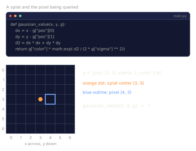
3. A splat in main.py has pos (3, 3), sigma 1, and color 0.6. What does gaussian_value return at pixel (4, 3), to two decimals?Apply
The gaussian_value source code above a 7 by 7 pixel grid. The splat center at (3, 3) is an orange dot and the pixel at (4, 3) is outlined in blue. Beside it are the splat values pos (3, 3), sigma 1, color 0.6, and the call gaussian_value(4, 3, g) equals a question mark.
Code copied from main.py.
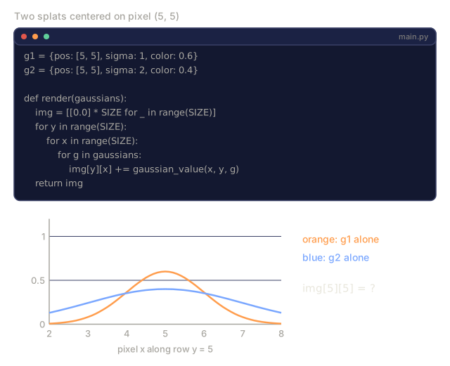
4. Two splats in main.py are both centered on pixel (5, 5). One has color 0.6 and sigma 1, the other color 0.4 and sigma 2. What does render put at (5, 5)?Apply
The two splat definitions and the render function from main.py, above a chart of each splat's own value along row 5: an orange curve peaking at 0.6 with sigma 1 and a wider blue curve peaking at 0.4 with sigma 2, both centered on pixel 5. A label asks for img[5][5].
Curves computed from the stem's numbers; code copied from main.py.
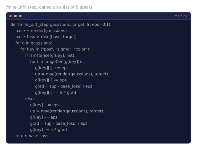
5. With 8 splats, how many full renders does one call to finite_diff_step perform?Apply
The full source of finite_diff_step from main.py, with its nested loops over each splat and each of the keys pos, sigma and color.
Copied from main.py. The question uses 8 splats.
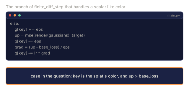
6. In finite_diff_step, nudging a splat's color up by eps makes the loss larger. What does the step then do to that color?Apply
Six lines of main.py: the else branch that nudges g[key] by eps, computes up, undoes the nudge, computes grad as (up - base_loss) / eps, and updates g[key]. A highlighted box states the case: key is color and up is greater than base_loss.
Code copied from main.py.
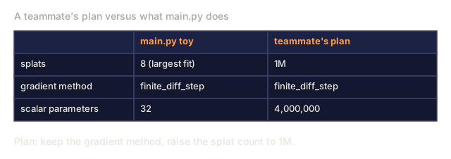
7. A teammate wants to keep main.py's gradient method and just raise the splat count to 1M for a real scene. What goes wrong?Analyze
A table comparing the main.py toy with a teammate's plan: splats 8 versus 1M, gradient method finite_diff_step in both, scalar parameters (4 per splat) 32 versus 4,000,000.
Toy values from main.py; the plan is the one in the question.

Pitfalls

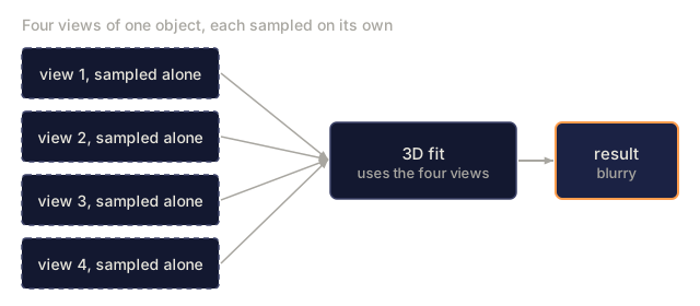
  • View inconsistency. Generate 4 views independently and they can disagree about the object's structure, which leaves the 3D fit blurry. Fix: multi-view diffusion with shared attention.
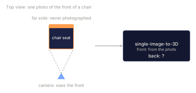
  • Back-side hallucination. Single-image → 3D has to invent the unseen side, and quality varies wildly.
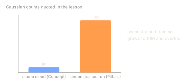
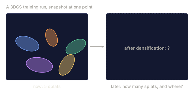
  • Gaussian splat explosion. Unconstrained training can grow to 10M splats and overfit. You need the densification and pruning heuristics from the original 3D-GS paper.
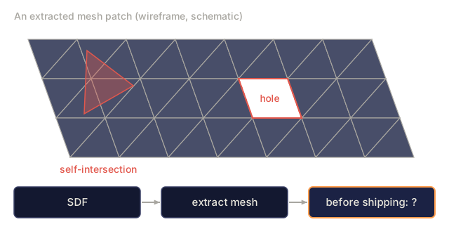
  • Topology issues. Meshes from implicit fields (SDFs) often have holes or self-intersections. Run a remesher (e.g. Blender's voxel remesh) before shipping.
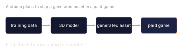
  • License of training data. Objaverse has mixed licenses, and what you can use commercially varies per model.
Check: Pitfalls0/6
1. What is densification in 3D Gaussian Splatting training?Define
Two panels. The left shows a snapshot of five translucent splats during 3D Gaussian Splatting training. The right is an empty dashed panel labelled after densification, with a question mark.
Illustrative: five splats drawn by hand to show the training state, not real training output.
2. Four views of one object are generated independently and the 3D fit comes out blurry. Why, and what fixes it?Analyze
Four dashed boxes labelled view 1 to view 4, each sampled alone, all with arrows into a 3D fit box, which leads to a highlighted result box marked blurry.
Schematic of the stem's setup.
3. A single-image-to-3D model is shown only the front of a chair. What problem do Pitfalls warn about for the back?Analyze
A top-down sketch of a chair with a camera facing its front, and a note that the far side was never photographed. An arrow leads to a single-image-to-3D box that lists front: from the photo and back: question mark.
Schematic of the stem's setup.
4. Unconstrained 3DGS training grows to 10M splats and overfits. What do Pitfalls say you need?Analyze
Two bars of Gaussian counts: about 1 million for a scene cloud in the Concept section, and 10 million for an unconstrained training run that overfits.
Figures quoted from the lesson.
5. A mesh extracted from an SDF has holes and self-intersections. What do Pitfalls recommend before shipping?Analyze
A wireframe triangle mesh patch with one missing quad labelled hole and one translucent red triangle cutting through the surface labelled self-intersection. Below, a flow: SDF, extract mesh, then a highlighted box reading before shipping, question mark.
Schematic mesh drawn by the script, not extracted from a real SDF.
6. A studio wants to ship a generated 3D asset in a paid game. What should it check about the model first?Design
A flow of four boxes: training data, 3D model, generated asset, paid game. Below, the line first check before using the model, question mark.
Schematic of the question's situation.

Use It

Task2026 pick
Scene reconstruction from photosGaussian splatting (3DGS, Gsplat, Scaniverse)
Text-to-3D object for gamesMeshy 4 or Rodin Gen-1.5 (PBR output)
Image-to-3DHunyuan3D 2.0, TripoSR, InstantMesh
Novel-view synthesis from few imagesCAT3D, SV3D
Dynamic scene reconstruction4D Gaussian Splatting
Avatar / clothed humanGaussian Avatar, HUGS
Research / SOTAWhatever dropped last week

For production 3D in a game or e-commerce pipeline, Meshy 4 and Rodin Gen-1.5 output PBR meshes that go straight into Unity / Unreal.
Check: Use It0/3
1. What is a PBR (physically-based rendering) material?Define
Three boxes joined by arrows: Meshy 4 or Rodin Gen-1.5, then a highlighted PBR mesh, then Unity or Unreal as the game engine.
Taken from the lesson's Use It section.
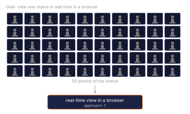
2. You have 50 photos of a statue and want to view it in real time in a browser. Which approach fits best?Apply
A grid of fifty small photo tiles, each showing a statue on a base, labelled 50 photos of the statue, with an arrow down to a highlighted box reading real-time view in a browser, approach: question mark.
Tiles are pictograms, not the real photos.
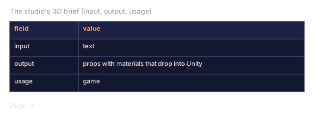
3. A game studio needs text-to-3D props with materials that drop straight into Unity. Which pick fits?Design
A three-field brief: input is text, output is props with materials that drop into Unity, usage is game. Below it, Pick: question mark.
Field names follow the lesson's Ship It brief; values come from the question.

Ship It

Save outputs/skill-3d-pipeline.md. The skill takes a 3D brief (input: text, one image, or a few images; output: mesh, splat, or NeRF; usage: render, game, or VR) and returns a pipeline (multi-view diffusion plus fit, or a direct mesh model), a base model, an iteration budget, topology post-processing, and the material channels needed.

Author's Note

I'd run main.py before touching a real splatting codebase. It fits 2, 4, and 8 splats to a 12x12 image and prints the final MSE plus an ASCII render for each. After 30 steps the loss only falls from about 0.060 to about 0.037, and the renders are still rough (the 8-splat one has stray blobs in the upper right), so what you see is the fit improving with more splats, not a clean match. Nothing in it needs a GPU or a library.

The gradient code is the part to read slowly. finite_diff_step perturbs each position, sigma, and color by eps, re-renders the whole image, and uses the change in loss as the gradient. That is expensive, and it only works because the image is tiny. A 3D-GS trainer gets the same quantity from a differentiable renderer in one backward pass, which is what makes millions of splats tractable.

I'd also keep the toy in proportion. It has no depth sorting, no alpha-compositing, no densification or pruning, and no camera, so it says nothing about the Pitfalls above. It does show the loop that everything else here is built on: render, compare to the target, nudge the parameters.

Exercises

  1. Easy. In code/main.py, change the for n in [2, 4, 8] loop to use 4, 16, 64 Gaussians. Report final MSE vs target.
  2. Medium. Extend to color Gaussians (RGB). Confirm reconstruction matches the target color pattern.
  3. Hard. Using gsplat or Nerfstudio, reconstruct a real object from a 50-photo capture. Report fit time and final SSIM on held-out views.

Key Terms

TermWhat people sayWhat it actually means
3D Gaussian Splatting"3DGS"Scene as a cloud of 3D Gaussians; differentiable alpha-composite render.
NeRF"Neural radiance field"MLP that outputs color + density at a 3D point; render by ray integration.
Triplane"Three 2-D planes"Factor 3D into three 2-D axis-aligned feature grids; cheaper than volumetric.
SDS"Score distillation sampling"Train 3D model by using 2D-diffusion score as pseudo-gradient.
Multi-view diffusion"Many views at once"Diffusion model that outputs a batch of consistent camera views.
PBR"Physically-based rendering"Material with albedo, roughness, metallic, normal channels.
Densification"Grow splats"3DGS training heuristic: split / clone splats in high-gradient regions.

Production note: 3D has no shared substrate yet

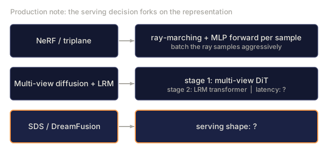
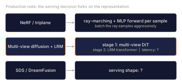
Image has latent diffusion and DiT, and video has the spatiotemporal DiT. 3D has no single dominant runtime in 2026, so the production decision tree forks on the representation:

  • NeRF / triplane. Inference is ray-marching plus an MLP forward per sample. A 512² render needs millions of MLP forwards, so batch the ray samples aggressively. SDPA/xformers applies.
  • Multi-view diffusion + LRM reconstruction. Two stages. Stage 1 (multi-view DiT) is a diffusion server just like Lesson 07. Stage 2 (LRM transformer) is a one-shot forward pass over the views. The latency profile is "diffusion + one-shot", so pick serving primitives per stage.
  • SDS / DreamFusion. This is per-asset optimization, not inference. Build jobs, not request handlers.

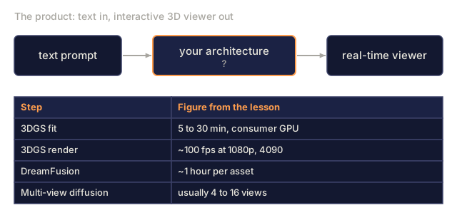
For most 2026 products, run a multi-view diffusion model on request, reconstruct to 3DGS asynchronously, and serve the 3DGS for real-time viewing. That splits the workload cleanly between a fast GPU-inference server and a slow offline optimizer.
Check: Production note: 3D has no shared substrate yet0/3
1. Why does the Production note say SDS/DreamFusion belongs in a job queue instead of a request handler?Explain
Three rows pairing a representation with a serving shape. NeRF or triplane: ray-marching plus an MLP forward per sample. Multi-view diffusion plus LRM: stage 1 multi-view DiT, stage 2 LRM transformer. SDS or DreamFusion, highlighted: serving shape is a question mark.
Rows summarize the lesson's Production note; two entries are hidden.
2. How does the Production note describe the latency profile of multi-view diffusion plus LRM?Explain
Three rows pairing a representation with a serving shape. Multi-view diffusion plus LRM, highlighted, lists stage 1 multi-view DiT and stage 2 LRM transformer with latency marked as a question mark. The NeRF row gives ray-marching plus an MLP forward per sample, and the SDS row is a question mark.
Rows summarize the lesson's Production note; two entries are hidden.
3. You must offer text-to-3D with a real-time viewer. Which architecture matches the recommended split of workloads?Design
A flow from text prompt through a highlighted box labelled your architecture, question mark, to a real-time viewer. Below, a table of lesson figures: 3DGS fit 5 to 30 minutes on a consumer GPU, 3DGS render about 100 fps at 1080p on a 4090, DreamFusion about 1 hour per asset, multi-view diffusion usually 4 to 16 views.
Figures quoted from the lesson.

Further Reading

Code

Ships With