Semantic Segmentation — U-Net
Segmentation is classification at every pixel. U-Net solved it by pairing a downsampling encoder with an upsampling decoder, then wiring skip connections between them so detail survives the round trip.
Learning Objectives
- Distinguish semantic, instance, and panoptic segmentation and pick the right task for a given problem
- Build a U-Net from scratch in PyTorch with encoder blocks, a bottleneck, an upsampling decoder, and skip connections
- Implement pixel-wise cross-entropy, Dice loss, and the combined loss that is the current default for medical and industrial segmentation
- Read IoU and Dice metrics per class and diagnose whether a bad score comes from small-object recall, boundary accuracy, or class imbalance
The Problem
Classification outputs one label per image. Detection outputs a handful of boxes. Segmentation outputs one label per pixel: for an H x W input, the output is a full H x W tensor (semantic) or H x W x N_instances (instance). That's millions of predictions per image, not one.
This is why segmentation runs almost every dense-prediction product in vision: medical imaging (tumor masks), autonomous driving (road, lane, obstacle), satellite (building footprints, crop boundaries), document parsing (layout zones), robotics (graspable regions). None of those tasks can be solved with a box around the object. They need the silhouette.
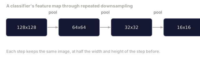
The hard part here is architectural, not conceptual: the network needs the global context of an image (what kind of scene is this) and the local pixel detail (which exact pixel is road versus pavement) at the same time. A standard CNN compresses spatially to gain that context, and the compression is exactly what throws the detail away. U-Net was the design that kept both.
The Concept
Semantic vs instance vs panoptic

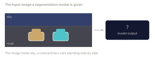
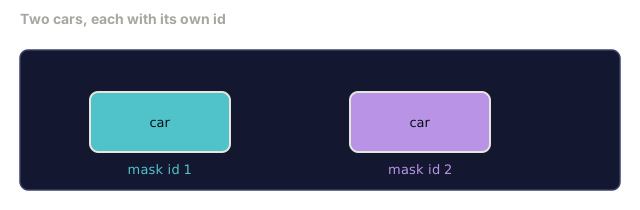
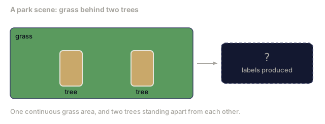
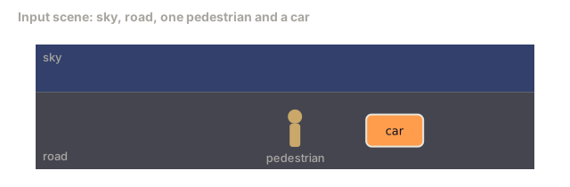
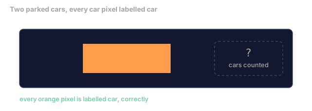
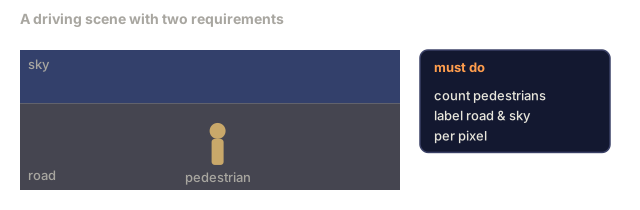
- Semantic segmentation says "this pixel is road, that pixel is car." Two cars sitting next to each other collapse into one blob.
- Instance segmentation says "this pixel is car #3, that pixel is car #5," and ignores background "stuff" (sky, road, grass) entirely.
- Panoptic segmentation unifies both: every pixel gets a class label, every instance also gets a unique id, so stuff and things are both segmented.
This lesson covers semantic segmentation. The next one, on Mask R-CNN, covers instance.
The U-Net shape

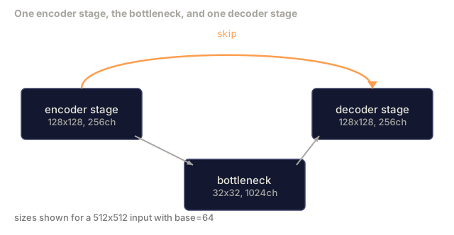
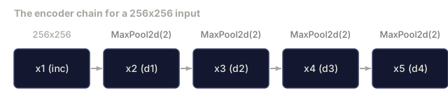
The encoder halves spatial resolution four times and doubles the channel count each time. The decoder mirrors that in reverse: doubling resolution and halving channels at every step. Skip connections concatenate the encoder's features into the decoder at each matching resolution, and a final 1x1 conv maps 64 -> num_classes at full resolution.
Skip connections exist because the decoder, by the time it has to output pixel-level predictions, has only seen small feature maps. Without them it can't localize edges accurately, because that spatial detail was compressed away going down the encoder. The skips hand back the high-resolution features the encoder computed on the way down, so the decoder has both the coarse context and the fine detail it needs.
Transposed vs bilinear upsample
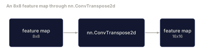
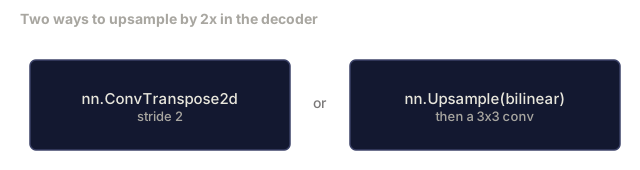
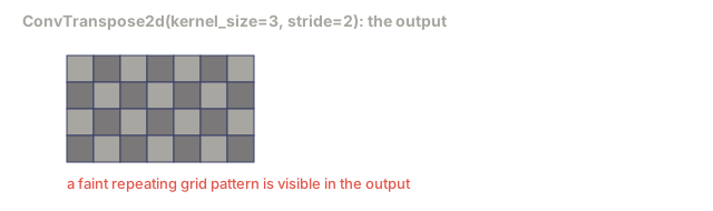
The decoder has to expand spatial dimensions, and there are two common ways to do it. Transposed convolution (nn.ConvTranspose2d) is a learnable upsample and was the original U-Net's choice, but it can produce checkerboard artifacts when stride and kernel size don't divide evenly. Bilinear upsample followed by a 3x3 conv is smoother, uses fewer parameters, produces fewer artifacts, and is the modern default.
Both show up in real codebases. For a first U-Net, bilinear is the safer choice.
Cross-entropy on a pixel grid
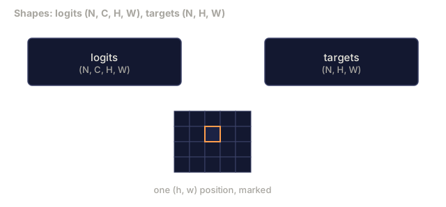
For semantic segmentation with C classes, the model output is (N, C, H, W). The target is (N, H, W) with integer class IDs. Cross-entropy is identical to the classification case, just applied at every spatial position:
Loss = mean over (n, h, w) of -log( softmax(logits[n, :, h, w])[target[n, h, w]] )
F.cross_entropy in PyTorch handles this shape natively. No reshape needed.
Dice loss and why you need it
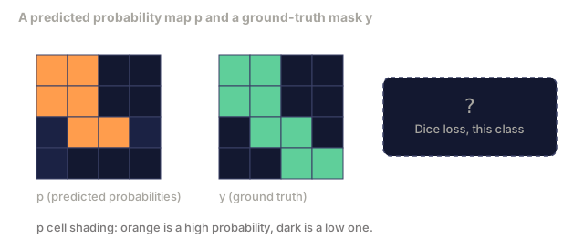
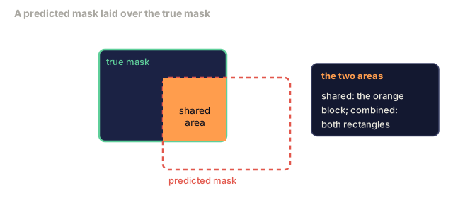
Dice loss directly optimizes the overlap between the predicted and true mask:
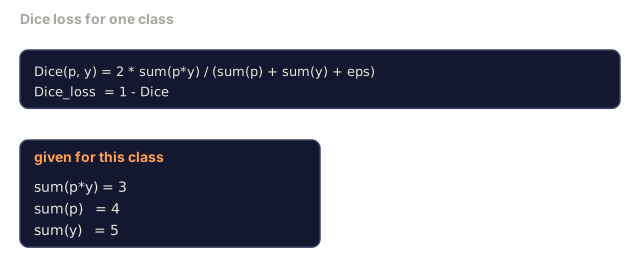
Dice(p, y) = 2 * sum(p * y) / (sum(p) + sum(y) + epsilon)
Dice_loss = 1 - Dice
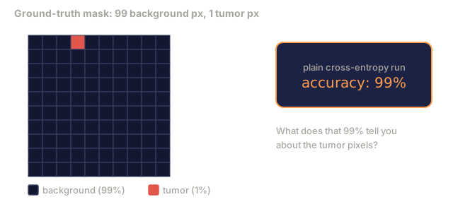
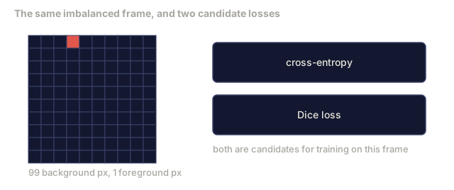
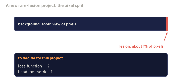
where p is the sigmoid/softmax probability map for a class and y is the binary ground-truth mask. The loss hits zero only when the overlap is perfect, and because it's ratio-based, class imbalance doesn't affect it. That matters because cross-entropy treats every pixel equally, which falls apart when one class dominates the frame (medical imaging: 99% background, 1% tumor); a network can hit 99% accuracy by predicting background everywhere and still be completely useless.
In practice, use the combined loss:
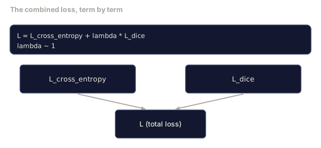
L = L_cross_entropy + lambda * L_dice (lambda ~ 1)
Cross-entropy gives stable gradients early in training; Dice spends the tail end of training actually matching the mask shape. This combination is the medical-imaging default, and it's hard to beat on any class-imbalanced dataset.
Evaluation metrics
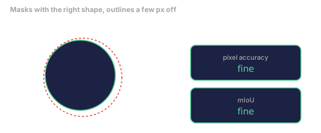
- Pixel accuracy: the percent of pixels predicted correctly. Cheap to compute, and just as broken on imbalanced data as plain accuracy is in classification.
- IoU per class, intersection over union for each class's mask, averaged across classes to get mIoU.
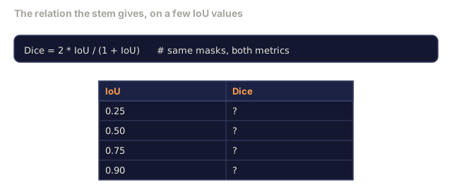
- Dice (F1 on pixels) is similar to IoU (
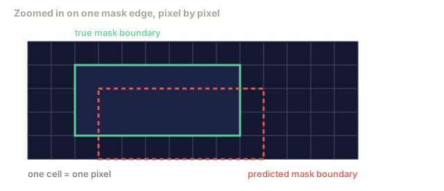
Dice = 2 * IoU / (1 + IoU)); medical imaging tends to report Dice, driving-scene work tends to report IoU, and the two are monotonically related, so it rarely matters which one you pick. - Boundary F1 measures how close predicted boundaries land to the ground-truth boundaries, penalizing even small shifts. It matters most for high-precision tasks like semiconductor inspection.
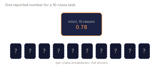
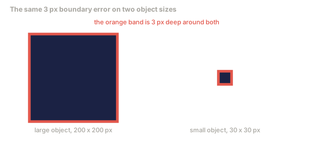
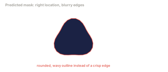
Report IoU per class, not just the mean. A mIoU of 0.78 can hide one class sitting at 15% while nine others sit at 85%. Small objects take the biggest hit here: a handful of missed boundary pixels is a much larger fraction of a small object's area than a large one, so a genuinely well-trained detector can still post its lowest IoU on the smallest class.
Input resolution trade-off
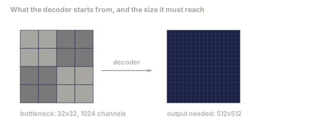
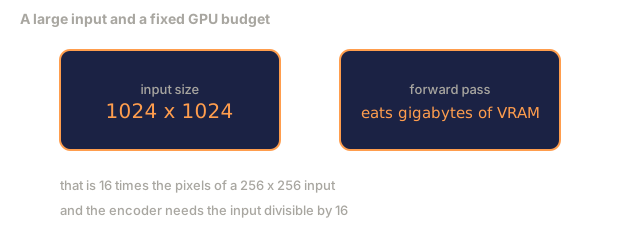
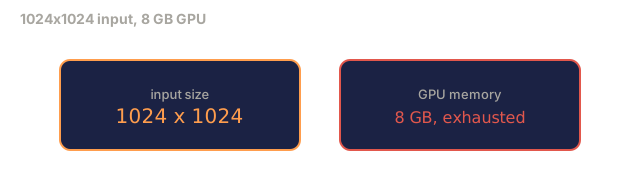
U-Net's encoder halves resolution four times, so the input has to be divisible by 16. Medical images often run 512x512 or 1024x1024; autonomous-driving crops run 2048x1024. Memory cost scales with H * W * C_max, and at 1024x1024 with 1024 bottleneck channels, the forward pass alone already eats gigabytes of VRAM.
There are two standard workarounds. Tile the input: process 256x256 tiles with overlap, then stitch the predictions back together. Or replace the bottleneck with dilated convolutions that keep spatial resolution higher while widening the receptive field, which is what the DeepLab family does.
For a first model, a 256x256 input with a 64-channel-base U-Net trains comfortably on 8 GB of VRAM.
Build It
Step 1: Encoder block
Two 3x3 convs with batch norm and ReLU. The first conv changes channel count; the second keeps it.
import torch
import torch.nn as nn
import torch.nn.functional as F

class DoubleConv(nn.Module):
    def __init__(self, in_c, out_c):
        super().__init__()
        self.net = nn.Sequential(
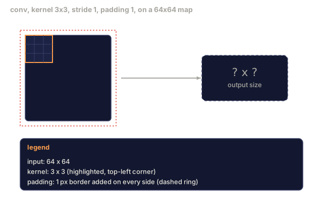
            nn.Conv2d(in_c, out_c, kernel_size=3, padding=1, bias=False),
            nn.BatchNorm2d(out_c),
            nn.ReLU(inplace=True),
            nn.Conv2d(out_c, out_c, kernel_size=3, padding=1, bias=False),
            nn.BatchNorm2d(out_c),
            nn.ReLU(inplace=True),
        )

    def forward(self, x):
        return self.net(x)
This block is reused throughout. bias=False because BN's beta handles the bias.
Step 2: Down and up blocks
class Down(nn.Module):
    def __init__(self, in_c, out_c):
        super().__init__()
        self.net = nn.Sequential(
            nn.MaxPool2d(2),
            DoubleConv(in_c, out_c),
        )

    def forward(self, x):
        return self.net(x)


class Up(nn.Module):
    def __init__(self, in_c, out_c):
        super().__init__()
        self.up = nn.Upsample(scale_factor=2, mode="bilinear", align_corners=False)
        self.conv = DoubleConv(in_c, out_c)

    def forward(self, x, skip):
        x = self.up(x)
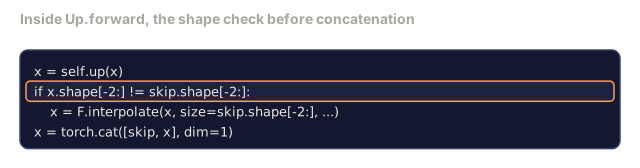
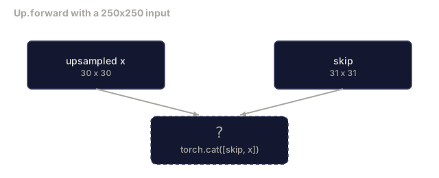
        if x.shape[-2:] != skip.shape[-2:]:
            x = F.interpolate(x, size=skip.shape[-2:], mode="bilinear", align_corners=False)
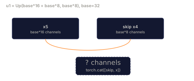
        x = torch.cat([skip, x], dim=1)
        return self.conv(x)
The spatial-only shape check (shape[-2:]) handles inputs whose dimensions are not divisible by 16; a safe F.interpolate aligns the tensor before the concat. Comparing the full shape would also trigger on channel-count differences, which should be a loud error, not a silent interpolate.
Step 3: The U-Net
class UNet(nn.Module):
    def __init__(self, in_channels=3, num_classes=2, base=64):
        super().__init__()
        self.inc = DoubleConv(in_channels, base)
        self.d1 = Down(base, base * 2)
        self.d2 = Down(base * 2, base * 4)
        self.d3 = Down(base * 4, base * 8)
        self.d4 = Down(base * 8, base * 16)
        self.u1 = Up(base * 16 + base * 8, base * 8)
        self.u2 = Up(base * 8 + base * 4, base * 4)
        self.u3 = Up(base * 4 + base * 2, base * 2)
        self.u4 = Up(base * 2 + base, base)
        self.outc = nn.Conv2d(base, num_classes, kernel_size=1)

    def forward(self, x):
        x1 = self.inc(x)
        x2 = self.d1(x1)
        x3 = self.d2(x2)
        x4 = self.d3(x3)
        x5 = self.d4(x4)
        x = self.u1(x5, x4)
        x = self.u2(x, x3)
        x = self.u3(x, x2)
        x = self.u4(x, x1)
        return self.outc(x)

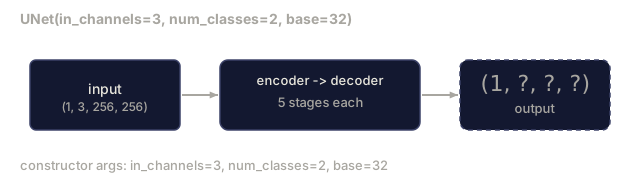
net = UNet(in_channels=3, num_classes=2, base=32)
x = torch.randn(1, 3, 256, 256)
print(f"output: {net(x).shape}")
print(f"params: {sum(p.numel() for p in net.parameters()):,}")
Output shape is (1, 2, 256, 256): same spatial size as the input, with num_classes channels instead of 3. About 7.7M parameters at base=32.
Step 4: Losses
def dice_loss(logits, targets, num_classes, eps=1e-6):
    probs = F.softmax(logits, dim=1)
    targets_one_hot = F.one_hot(targets, num_classes).permute(0, 3, 1, 2).float()
    dims = (0, 2, 3)
    intersection = (probs * targets_one_hot).sum(dim=dims)
    denom = probs.sum(dim=dims) + targets_one_hot.sum(dim=dims)
    dice = (2 * intersection + eps) / (denom + eps)
    return 1 - dice.mean()


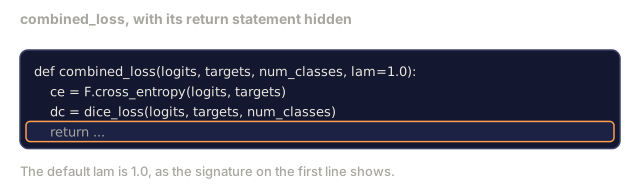
def combined_loss(logits, targets, num_classes, lam=1.0):
    ce = F.cross_entropy(logits, targets)
    dc = dice_loss(logits, targets, num_classes)
    return ce + lam * dc, {"ce": ce.item(), "dice": dc.item()}
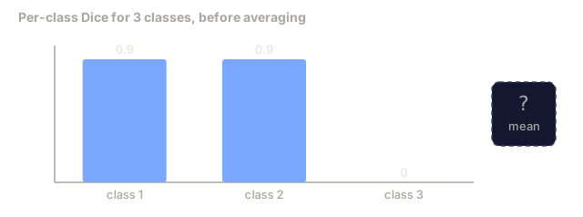
Dice is computed per class then averaged (macro Dice). The eps prevents division by zero on classes absent from the batch.
Step 5: IoU metric
@torch.no_grad()
def iou_per_class(logits, targets, num_classes):
    preds = logits.argmax(dim=1)
    ious = torch.zeros(num_classes)
    for c in range(num_classes):
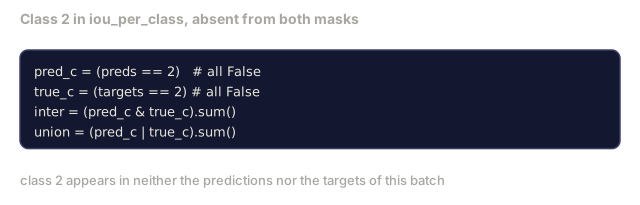
        pred_c = (preds == c)
        true_c = (targets == c)
        inter = (pred_c & true_c).sum().float()
        union = (pred_c | true_c).sum().float()
        ious[c] = (inter / union) if union > 0 else torch.tensor(float("nan"))
    return ious
Returns a vector of length C; nan marks classes absent from the batch, so don't average over those when computing mIoU.
Step 6: Synthetic dataset for end-to-end verification
Generate shapes on colored backgrounds so the network has to learn shape, not pixel color.
import numpy as np
from torch.utils.data import Dataset, DataLoader

def synthetic_segmentation(num_samples=200, size=64, seed=0):
    rng = np.random.default_rng(seed)
    images = np.zeros((num_samples, size, size, 3), dtype=np.float32)
    masks = np.zeros((num_samples, size, size), dtype=np.int64)
    for i in range(num_samples):
        bg = rng.uniform(0, 1, (3,))
        images[i] = bg
        masks[i] = 0
        num_shapes = rng.integers(1, 4)
        for _ in range(num_shapes):
            cls = int(rng.integers(1, 3))
            color = rng.uniform(0, 1, (3,))
            cx, cy = rng.integers(10, size - 10, size=2)
            r = int(rng.integers(4, 12))
            yy, xx = np.meshgrid(np.arange(size), np.arange(size), indexing="ij")
            if cls == 1:
                mask = (xx - cx) ** 2 + (yy - cy) ** 2 < r ** 2
            else:
                mask = (np.abs(xx - cx) < r) & (np.abs(yy - cy) < r)
            images[i][mask] = color
            masks[i][mask] = cls
        images[i] += rng.normal(0, 0.02, images[i].shape)
        images[i] = np.clip(images[i], 0, 1)
    return images, masks


class SegDataset(Dataset):
    def __init__(self, images, masks):
        self.images = images
        self.masks = masks

    def __len__(self):
        return len(self.images)

    def __getitem__(self, i):
        img = torch.from_numpy(self.images[i]).permute(2, 0, 1).float()
        mask = torch.from_numpy(self.masks[i]).long()
        return img, mask
Three classes: background (0), circles (1), squares (2). The network must learn to distinguish shape.
Step 7: Training loop
def train_one_epoch(model, loader, optimizer, device, num_classes):
    model.train()
    loss_sum, total = 0.0, 0
    iou_sum = torch.zeros(num_classes)
    for x, y in loader:
        x, y = x.to(device), y.to(device)
        logits = model(x)
        loss, _ = combined_loss(logits, y, num_classes)
        optimizer.zero_grad()
        loss.backward()
        optimizer.step()
        loss_sum += loss.item() * x.size(0)
        total += x.size(0)
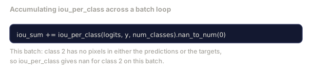
        iou_sum += iou_per_class(logits, y, num_classes).nan_to_num(0)
    return loss_sum / total, iou_sum / len(loader)
Run this for 10-30 epochs on the synthetic dataset and watch mIoU climb past 0.9 for the shape classes. Note the nan_to_num(0) treats classes absent from a batch as zero; for accurate per-class IoU, mask by presence and use torch.nanmean across batches at evaluation time rather than averaging here.
Use It
For production, segmentation_models_pytorch ("smp") wraps every standard segmentation architecture with any torchvision or timm backbone. It's three lines:
import segmentation_models_pytorch as smp

model = smp.Unet(
    encoder_name="resnet34",
    encoder_weights="imagenet",
    in_channels=3,
    classes=3,
)
Also worth knowing for real work:
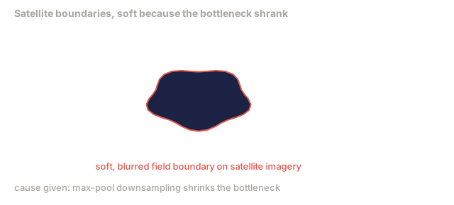
- DeepLabV3+ swaps max-pool-based downsampling for dilated convs, so the bottleneck keeps its resolution and boundaries come out sharper on satellite and driving data.
- SegFormer replaces the conv encoder with a hierarchical transformer and has ranked near the top of several segmentation benchmarks.
- Mask2Former and OneFormer go further and unify semantic, instance, and panoptic segmentation into one architecture.
All three drop in as replacements inside smp or transformers, using the same data loader.
Ship It
This lesson produces:
outputs/prompt-segmentation-task-picker.md: a prompt that picks between semantic, instance, and panoptic segmentation and names the architecture for a given task.outputs/skill-segmentation-mask-inspector.md: a skill that reports class distribution and predicted-mask statistics, and flags the classes that are under-predicted or have blurred boundaries.
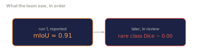
The most wasted debugging time I've seen on a segmentation project has nothing to do with the architecture. A team ships a U-Net trained on plain cross-entropy, watches a strong mIoU come in, and doesn't notice their rare class has a Dice score near zero until someone asks about it directly in a review. Add Dice to the loss from day one, even before you think you need it, and report IoU per class starting with your very first training run. It costs a few extra lines of code and saves you an awkward conversation three weeks later.
The other thing worth knowing before you hit it: bilinear upsampling beat transposed convolutions for a mundane reason, not a clever one. Checkerboard artifacts show up when a learnable upsample's receptive fields overlap unevenly across output positions, and once you've stared at a prediction with a faint grid baked into it, you stop reaching for ConvTranspose2d by default.
Exercises
- (Easy) Implement
bce_dice_lossfor a binary segmentation task (foreground vs background). Verify on a synthetic two-class dataset that the combined loss converges faster than BCE alone when the foreground is 5% of pixels. - (Medium) Replace the
nn.Upsample + convup-block with ann.ConvTranspose2dup-block. Train both on the synthetic dataset and compare mIoU. Observe where checkerboard artifacts appear in the transposed-conv version. - (Hard) Take a real segmentation dataset (Oxford-IIIT Pets, Cityscapes mini split, or a medical subset) and train the U-Net to within 2 IoU points of the
smp.Unetreference. Report per-class IoU and identify which classes benefit most from adding Dice to the loss.
Key Terms
| Term | What people say | What it actually means |
|---|---|---|
| Semantic segmentation | "Label every pixel" | Per-pixel classification into C classes; instances of the same class merge |
| Instance segmentation | "Label every object" | Separates distinct instances of the same class; foreground-only |
| Panoptic segmentation | "Semantic + instance" | Every pixel gets a class; every thing instance also gets a unique id |
| Skip connection | "U-Net bridge" | Concatenation of encoder features into matching-resolution decoder features; preserves high-frequency detail |
| Transposed conv | "Deconvolution" | Learnable upsampling; can produce checkerboard artifacts |
| Dice loss | "Overlap loss" | 1 - 2 |
| mIoU | "Mean intersection over union" | Average IoU across classes; the community-standard metric for segmentation |
| Boundary F1 | "Boundary accuracy" | F1 score computed on boundary pixels only; matters for precision-critical tasks |
Further Reading
- U-Net: Convolutional Networks for Biomedical Image Segmentation (Ronneberger et al., 2015): the original paper — the figure everyone copies is on page 2.
- Fully Convolutional Networks (Long et al., 2015): the paper that first made segmentation an end-to-end conv problem.
- segmentation_models_pytorch: the reference for production segmentation, with every standard architecture and every standard loss already implemented.
- Lessons learned from training SOTA segmentation (kaggle.com competitions): a walkthrough of why TTA, pseudo-labeling, and class weights matter on real data.
Code
- main.py (python, 183 lines)