Multi-Token Prediction (MTP)
Autoregressive LLMs from GPT-2 to Llama 3 train on one loss per position: predict the next token. DeepSeek-V3 added a second loss per position: predict the token after that. The extra 14B of parameters (on a 671B model) pushed gradient back into the main model, and the trained MTP heads were repurposed at inference as speculative-decoding drafters with 80%+ acceptance. The reported result was 1.8× generation throughput at inference. This lesson builds the sequential MTP module from the DeepSeek technical report, computes the loss and the shared-head parameter layout, and explains why MTP keeps the causal chain while Gloeckle et al.'s original parallel MTP broke it.
Learning Objectives
- State the MTP training objective and derive the joint loss across prediction depths.
- Explain the difference between Gloeckle et al.'s parallel MTP heads (2024) and DeepSeek-V3's sequential MTP modules and why the sequential design preserves the causal chain.
- Compute the parameter and memory overhead of adding MTP modules to a pre-training run.
- Implement one MTP module from scratch: the shared embedding, the per-depth transformer block, the projection, and the shared output head.
The Problem
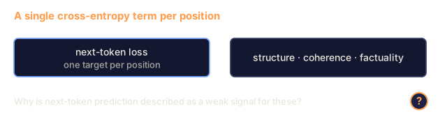
Next-token prediction is the standard LLM training objective. Every hidden state is supervised to predict exactly one thing: the immediately following token. That is a weak signal. Most of what matters in a sequence extends beyond one token: structure, coherence, factuality, the flow of an arithmetic problem. The model has to pick all of that up by accumulating one-token signals over trillions of tokens.
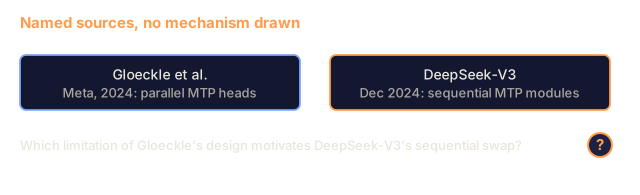
MTP asks: what if every hidden state were supervised to predict multiple future tokens at once? Gloeckle et al. (Meta, 2024) showed this helps. Their implementation put several independent output heads on top of the backbone, each predicting a different offset. The design is parallel and simple, but every head saw the same hidden state with no refinement between offsets. The predictions did not chain causally, so they could not serve as a speculative-decoding drafter.
DeepSeek-V3 (December 2024) re-designed MTP as sequential modules that keep the causal chain at each prediction depth. The model predicts t+1 from h_i^(0), then predicts t+2 from a new hidden state h_i^(1) that combines h_i^(0) with the E(t+1) embedding, and so on. Each depth is its own small transformer block. The shared embedding and shared output head keep parameter overhead modest. At DeepSeek-V3's scale that is 14B extra parameters across MTP modules on top of 671B main-model weights. About 2% overhead buys a denser training signal and a ready-made speculative-decoding draft at inference.
This lesson builds a single MTP module and the D-depth loss from scratch. The math is tidy, and the implementation is short enough to read in one sitting.
The Concept
The sequential MTP recipe
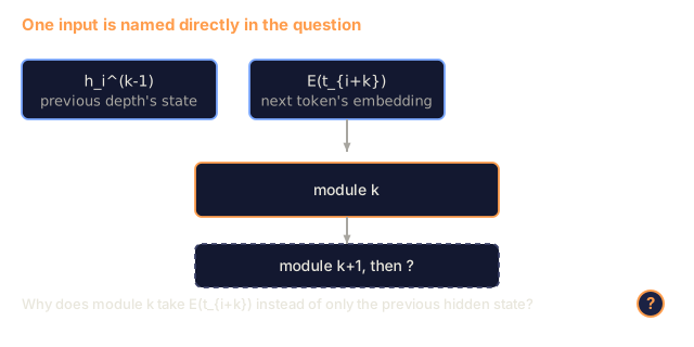
DeepSeek-V3 adds D MTP modules on top of the main model. Prediction depth k (for k = 1..D) predicts t_{i+k} given a prefix through position i. Depth 1 reads the backbone state h_i^(0). Module k builds the next state h_i^(k), which is what depth k+1 reads.
A note on numbering. In the formulas below, depth k reads h_i^(k-1), so depth 1 is the backbone's own next-token head and module k feeds depth k+1. The paper counts modules instead: its D = 1 is one extra module predicting t_{i+2}, which is depth 2 here. So the paper's D modules give D+1 depths in this numbering. In the speculative-decoding and parameter sections, "D=1 module" means the paper's first module (the one that predicts t_{i+2}), and "acceptance at depth 1" is a loose label for that same module's draft, not for the depth-1 head above. The toy in main.py builds D modules but reads only depths 1 to D, so its last module's output goes unused.
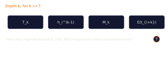
Module k consists of:
- A transformer block
T_kwith its own attention and MLP. - A projection matrix
M_kthat combines the previous-depth hidden state with the embedding of the next-depth ground-truth token. - The shared embedding
E(same as the main model). - The shared output head
Out(same as the main model).
At training, for a prefix through position i, the per-depth hidden state is:
h_i^(0) = main model backbone at position i
h_i^(k) = T_k( M_k * concat(RMSNorm(h_i^(k-1)), RMSNorm(E(t_{i+k}))) )   for k >= 1
The per-depth prediction is:
logits_{i+k} = Out(h_i^(k-1)) for k = 1..D
The per-depth loss is cross-entropy against the ground-truth t_{i+k}:
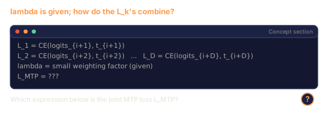
L_k = CE(logits_{i+k}, t_{i+k})
The joint loss across depths:
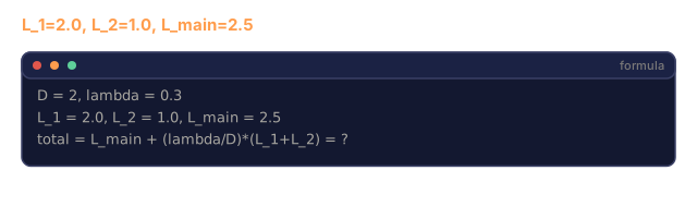
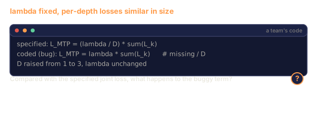
L_MTP = (lambda / D) * sum_{k=1..D} L_k
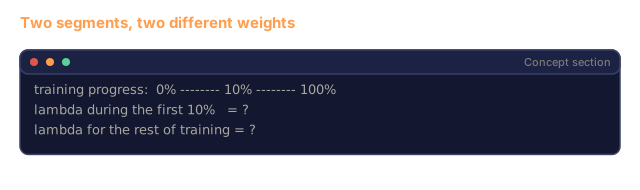
lambda is a small weighting factor. DeepSeek-V3 uses 0.3 for the first 10% of training and 0.1 afterward. The total training loss is L_main + L_MTP.
Why sequential, not parallel
Gloeckle's original parallel MTP had D output heads, each directly applied to h_i^(0). Each head predicts t_{i+k} from the same backbone hidden state. That trains fine, but the predictions are not conditioned on each other. head_1's output cannot help head_2 because the heads fire in parallel.
DeepSeek-V3's sequential design builds h_i^(k) from h_i^(k-1) plus the actual next-token embedding E(t_{i+k}). That preserves the causal chain: to predict t_{i+k+1}, the module at depth k+1 sees what was at t_{i+k}. This is the same shape as an autoregressive decoder consuming its own output, which is why the MTP modules can be used directly as speculative-decoding drafters.
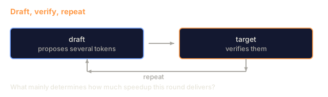
At inference: feed h_i^(k-1) and the drafted t_{i+k} into module k to build h_i^(k), then read Out(h_i^(k)) as the draft for t_{i+k+1}. Repeat. That is exactly an EAGLE-style draft, using the trained MTP module as the draft network. DeepSeek-V3 reports 80%+ acceptance on the first MTP module and ~1.8× speedup.
Parameter accounting
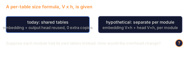
For a model with hidden h and vocabulary V:
- Main model: billions of parameters, plus one output head of size
V * h. - Shared output head: reuse the main model's head. No extra params.
- Shared embedding: reuse the main model's embedding. No extra params.
- Per-MTP module:
- Projection
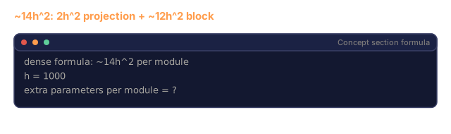
M_k:(2h) * h = 2h^2. - Transformer block
T_k: attention (4h^2for MHA) plus MLP (typically8h^2for SwiGLU with ratio 8/3). About12h^2per block.
- Projection
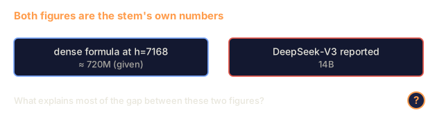
Total extra per module: ~14h^2. For DeepSeek-V3's h = 7168, D = 1 module: ~14 * 7168^2 = ~720M parameters on paper. DeepSeek-V3 reports 14B. The gap comes mostly from the MTP module's transformer block being MoE as well, which the dense formula does not count.
The speculative-decoding payoff
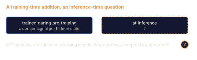
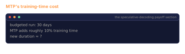
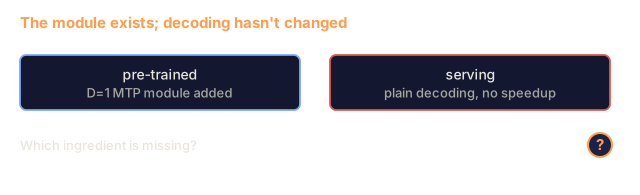
During pre-training, the MTP modules slow training by about 10% (more forward compute, extra loss). The payoff comes in two parts:
-
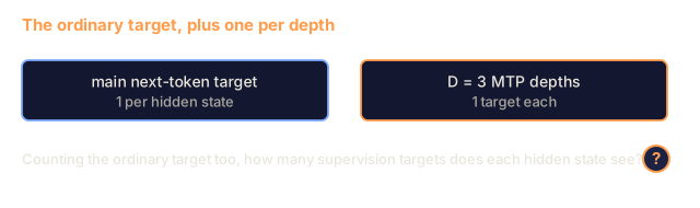
Denser training signal. Each hidden state sees D+1 supervision targets. DeepSeek-V3's ablations on MMLU, GSM8K, MATH, and HumanEval show improvements of a few percentage points.
-
A speculative-decoding draft at inference. The MTP module is already trained to predict the next few tokens. Repurposed as a draft network, it reaches 80%+ acceptance, and DeepSeek-V3 reports 1.8× throughput from it. The roughly 10% training-time cost is paid once, and the draft keeps paying back at every inference run.
Relation to EAGLE
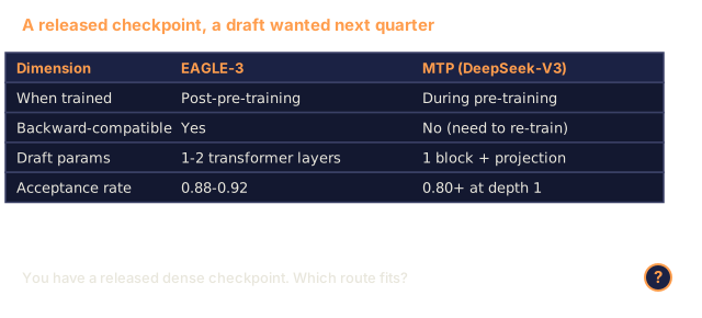
EAGLE trains a small draft model separately after pre-training. MTP bakes the draft into pre-training. The two reach similar acceptance rates through different pipelines:
| Dimension | EAGLE-3 | MTP (DeepSeek-V3) |
|---|---|---|
| When trained | Post-pre-training | During pre-training |
| Backward-compatible with existing weights | Yes | No (need to re-train) |
| Draft params | 1-2 transformer layers | 1 transformer block + projection |
| Acceptance rate | 0.88-0.92 | 0.80+ at depth 1 |
| Benefit beyond speedup | Speculative decoding only | Denser training signal + speedup |
Build It
code/main.py builds a single MTP module end to end: shared embedding, projection, transformer block, shared output head. It then computes the per-depth cross-entropy loss on a short synthetic sequence and prints the parameter count by component. A toy vocabulary of 32 tokens keeps the numbers readable.
Step 1: shared embedding table
One vocab_size x hidden table serves the main model and each MTP module at each depth. There is no second copy, only the same tensor. In main.py the output head is tied to it too: shared_head_logits computes E_v . hidden against the same table.
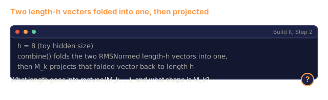
Step 2: the per-depth combination
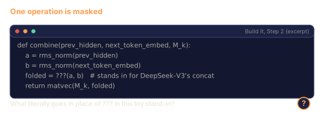
def combine(prev_hidden, next_token_embed, M_k):
    # concat along feature dim, then project down to hidden
    concat = rms_norm(prev_hidden) + rms_norm(next_token_embed)  # vector addition stand-in
    projected = matvec(M_k, concat)
    return projected
Real DeepSeek-V3 concatenates the two RMSNormed vectors to [2h] and projects with an h x 2h matrix. The toy uses vector addition for stdlib brevity.
Step 3: the transformer block at depth k
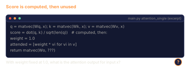
Attention plus MLP. The toy keeps the q/k/v/out projections and a SwiGLU MLP, both with residual connections, so the structure is visible without numpy. The attention is a single-token stand-in: it computes the score but applies a fixed weight of 1.0, so it reduces to Wo(Wv x). A full implementation attends over a KV cache and drops in at the same spot.
Step 4: the shared output head
Reuse the main model's output projection to get logits over the vocabulary.
Step 5: per-depth loss
Cross-entropy of softmax(logits) against the ground-truth token at offset k. Aggregate across depths with the lambda / D scaling factor.
Step 6: parameter accounting
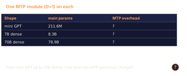
Print the parameter counts for the main model and the MTP modules, and the ratio of MTP extra to main-model size, for the toy and for a few real model shapes.
Use It
MTP is integrated into DeepSeek-V3 (December 2024) and the DeepSeek-R1 series. At inference:
- DeepSeek's own serving stack consumes MTP modules as speculative decoders out of the box.
- vLLM and SGLang have integration paths for DeepSeek-V3 MTP as of April 2026.
- AMD's ROCm SGLang tutorial shows a specific MTP speculative-decoding config with measured 1.8× speedup on the V3 checkpoint.
When to use MTP in a new pre-training run:
- You control the full pre-training pipeline and want a denser training signal.
- You plan to serve the model at scale and want a speculative-decoding draft without a separate training stage.
- Your hidden size is at least 4096. At 1B scale the overhead likely costs more than the gain returns.
When not to:
- Fine-tuning an existing pre-trained dense model. The MTP module is not trained.
- Research models where you want a clean baseline to compare against. MTP changes the architecture.
Ship It
This lesson produces outputs/skill-mtp-planner.md. Given a pre-training run specification (model size, data, compute), it returns a plan for integrating MTP: number of depths D, lambda schedule, memory overhead, and the inference-time speculative-decoding wiring.
I'd run main.py first and read the parameter table before the loss numbers. It prints the MTP overhead for the toy and for a few real shapes (mini GPT, 7B, 70B, DeepSeek-V3-shaped), and those percentages are what decide whether MTP is worth adding to a run.
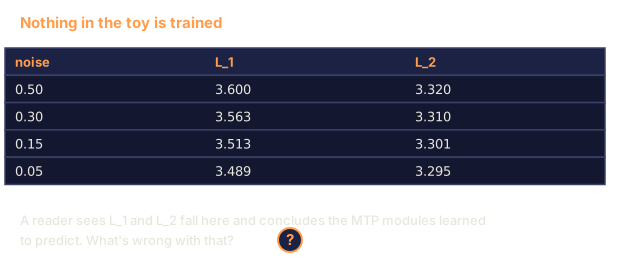
Be careful with what the loss numbers mean. Nothing in the toy is trained. The third printed section lowers the noise on the backbone hidden states by hand and re-evaluates, so L_1 and L_2 falling there shows that the loss responds to a better backbone, not that MTP learns anything. Exercise 1 is where you add a real signal.
The toy also simplifies the module more than the prose does. It adds the two RMSNormed vectors instead of concatenating them, so M_k is h x h rather than h x 2h, and the attention has a fixed weight of 1.0. Read mtp_forward for the order of operations, and keep the equations above for the real shapes. The loss loop in the toy runs D depths, so the state built by the last module is never read. In the full design it is the one that predicts t_{i+D+1}. My bet is that the sequential chain, where the depth-k module takes the ground-truth embedding of t_{i+k}, is the part worth rereading until it feels obvious.
Exercises
-
Run
code/main.py. Show the per-depth loss decreases monotonically as the synthetic signal strengthens. Modify the synthetic to use a fixed pattern and verify both depth-1 and depth-2 losses converge. -
Compute the parameter overhead for a dense 70B model (hidden 8192, 80 layers) with D=1 MTP module. Compare to the DeepSeek-V3 reported 14B overhead. Explain why DeepSeek's number is higher: the MTP transformer block inherits the same MoE structure, inflating the per-module parameter count.
-
Implement D=2 in the toy: add a second MTP module that takes h^(1) and
E(t_{i+2}), builds h^(2), and predictst_{i+3}from it. Verify the joint loss and the parameter accounting match the DeepSeek paper's equations 19-21. -
Switch the toy to parallel MTP (Gloeckle-style): add D output heads on top of the main hidden state, each predicting a different offset. Measure how the losses per depth compare to the sequential version on the same synthetic signal. The sequential version should produce lower depth-k loss for k > 1 because it conditions on the intermediate predictions.
-
Use the trained MTP module as an EAGLE-style draft: run module k on h^(k-1) and the drafted
t_{i+k}to proposet_{i+k+1}at inference. Measure the acceptance rate of these draft tokens against the main model's predictions on a held-out sequence. If you hit 50%+ on the toy, you have reproduced the empirical MTP-as-draft property.
Key Terms
| Term | What people say | What it actually means |
|---|---|---|
| MTP module | "Extra loss block" | A small transformer block plus projection that extends the hidden state by one depth, so a token one position further ahead can be predicted from it |
| Prediction depth | "Which offset" | The integer k such that depth k predicts t_{i+k} from h_i^(k-1), the state built by module k-1 (the backbone for k = 1), given a prefix through position i |
| Parallel MTP | "Gloeckle-style" | D independent heads on the same backbone hidden state, no conditional chain |
| Sequential MTP | "DeepSeek-V3 style" | Each module conditions on the previous depth's hidden state plus the next token's embedding; preserves causal chain |
| Shared output head | "Reuse the main head" | The MTP modules call the main model's LM head, not a separate output projection |
| Shared embedding | "Reuse the main table" | Same vocabulary embedding table is used everywhere; no duplicate parameters |
| Projection matrix M_k | "Combine hidden + next-token" | An h x 2h linear layer that folds the previous hidden state and the target-token embedding into the next depth's input |
| Joint loss L_MTP | "Averaged extra losses" | Arithmetic mean of per-depth cross-entropy losses, scaled by lambda |
| Acceptance rate at depth 1 | "How often MTP draft is right" | The rate at which the D=1 MTP module's top-1 prediction equals the main model's top-1 prediction; 80%+ on DeepSeek-V3 |
| Lambda weighting | "Extra-loss importance" | Per-depth scaling factor; 0.3 at start of training, 0.1 later on DeepSeek-V3 |
Further Reading
- DeepSeek-AI. DeepSeek-V3 Technical Report (arXiv:2412.19437): the full sequential MTP description (Section 2.2), including the joint-loss equations and the 1.8× speedup at inference
- Gloeckle et al., Better & Faster Large Language Models via Multi-token Prediction (arXiv:2404.19737): the parallel MTP baseline DeepSeek's design improves on
- DeepSeek-V3 model card on Hugging Face: 685B total (671B main + 14B MTP), deployment notes
- Leviathan et al., Fast Inference from Transformers via Speculative Decoding (arXiv:2211.17192): the speculative-decoding framework MTP fits into
- Li et al., EAGLE-3 (arXiv:2503.01840): EAGLE's 2025 draft architecture, the counterpart MTP competes with
Code
- main.py (python, 279 lines)