Hyperparameter Tuning
Hyperparameters are the knobs you set before training starts. Most of them barely move the outcome, so the real skill is finding the one or two that do and spending your search budget there.
Learning Objectives
- Implement grid search, random search, and Bayesian optimization from scratch and compare their sample efficiency
- Explain why random search outperforms grid search when most hyperparameters have low effective dimensionality
- Build a Bayesian optimization loop using a surrogate model and acquisition function to guide the search
- Design a hyperparameter tuning strategy that avoids overfitting the validation set through proper cross-validation
The Problem
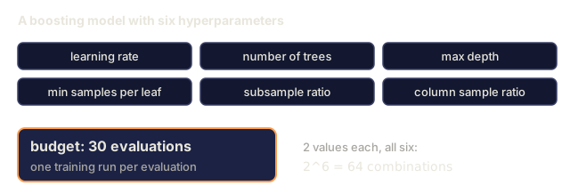
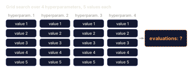
Your gradient boosting model has a learning rate, number of trees, max depth, min samples per leaf, subsample ratio, and column sample ratio. That's six hyperparameters. Give each five reasonable values and the grid balloons to 5^6 = 15,625 combinations. At 10 seconds per training run, trying them all costs 43 hours of compute.
Grid search is the obvious approach and the worst one at scale. Random search does better with less compute. Bayesian optimization does better still, because it learns from every evaluation instead of throwing the result away. Knowing which strategy fits your budget, and which hyperparameters actually move the needle, is the difference between an afternoon of tuning and a week of wasted GPU time.
The Concept
Parameters vs Hyperparameters
Parameters are learned during training (weights, biases, split thresholds). Hyperparameters are set before training starts and control how learning happens.
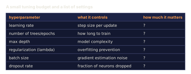
| Hyperparameter | What it controls | Typical range |
|---|---|---|
| Learning rate | Step size per update | 0.001 to 1.0 |
| Number of trees/epochs | How long to train | 10 to 10,000 |
| Max depth | Model complexity | 1 to 30 |
| Regularization (lambda) | Overfitting prevention | 0.0001 to 100 |
| Batch size | Gradient estimation noise | 16 to 512 |
| Dropout rate | Fraction of neurons dropped | 0.0 to 0.5 |
Grid Search
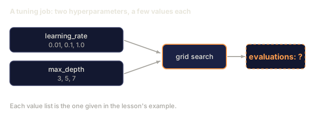
Grid search evaluates every combination of specified values. It is exhaustive and easy to understand, but scales exponentially with the number of hyperparameters.
Grid for 2 hyperparameters:

  learning_rate: [0.01, 0.1, 1.0]
  max_depth:     [3, 5, 7]

  Evaluations: 3 x 3 = 9 combinations

  (0.01, 3)  (0.01, 5)  (0.01, 7)
  (0.1,  3)  (0.1,  5)  (0.1,  7)
  (1.0,  3)  (1.0,  5)  (1.0,  7)
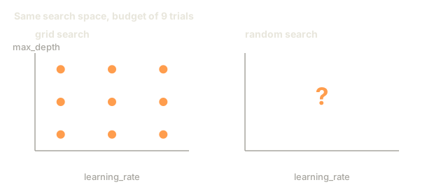
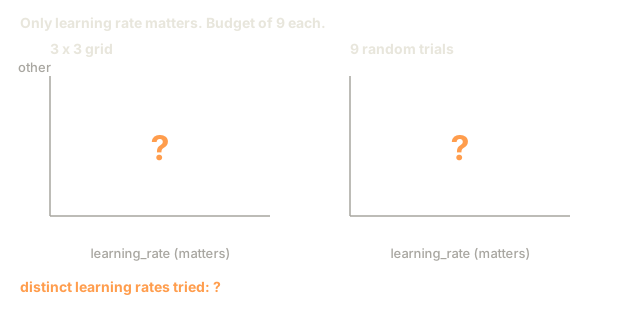
Grid search has a fundamental flaw: if one hyperparameter matters and the other does not, most evaluations are wasted. You get only 3 unique values of the important parameter from 9 evaluations.
Random Search
Random search samples hyperparameters from distributions instead of a grid. With the same budget of 9 evaluations, you get 9 unique values of each hyperparameter.

Why random beats grid (Bergstra & Bengio, 2012):
- Most hyperparameters have low effective dimensionality. Only 1-2 of 6 hyperparameters usually matter for a given problem.
- Grid search wastes evaluations on unimportant dimensions.
- Random search covers the important dimensions more densely for the same budget.
- At 60 random trials, you have a 95% chance of finding a point within 5% of the optimum (if one exists in the search space).
Bayesian Optimization
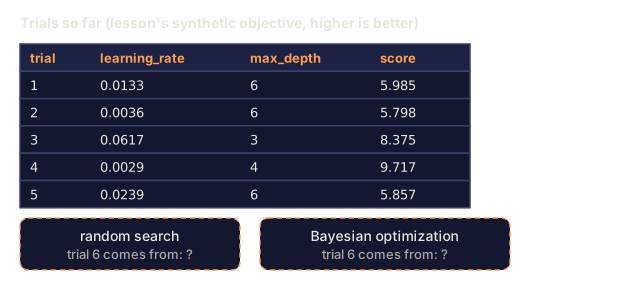
Bayesian optimization uses the results of past evaluations to decide where to search next. Random search can't do that: it doesn't learn that high learning rates cause divergence, or that depth 3 consistently beats depth 10, because every trial starts from scratch with no memory of what came before.

The two key components:
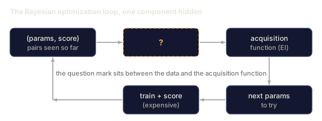
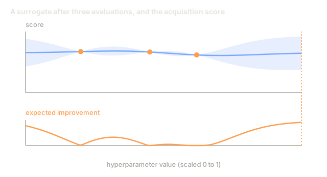
Surrogate model: A cheap-to-evaluate model (usually a Gaussian process) that approximates the expensive objective function. It gives both a prediction and an uncertainty estimate at any point in the search space.
Acquisition function: Decides where to evaluate next by balancing exploitation (search near known good points) and exploration (search where uncertainty is high). Common choices:
- Expected Improvement (EI): How much improvement over the current best do we expect at this point?
- Upper Confidence Bound (UCB): Prediction plus a multiple of uncertainty. Higher UCB means either promising or unexplored.
- Probability of Improvement (PI): What is the probability this point beats the current best?
Bayesian optimization typically finds better hyperparameters than random search with 2-5x fewer evaluations. The overhead of fitting the surrogate model is negligible compared to training the actual model.
Early Stopping
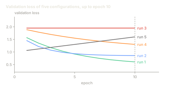
Early stopping, in the context of hyperparameter search, means not letting every training run finish: if a configuration is clearly bad after 10 epochs, kill it and move on.
Strategies:
- Patience-based: Stop if validation loss has not improved for N consecutive epochs
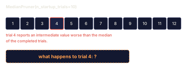
- Median pruning: Stop if the trial's intermediate result is worse than the median of completed trials at the same step
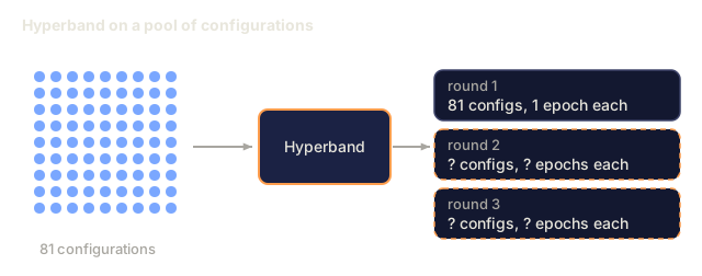
- Hyperband: Allocate small budgets to many configurations, then progressively increase budget for the best ones
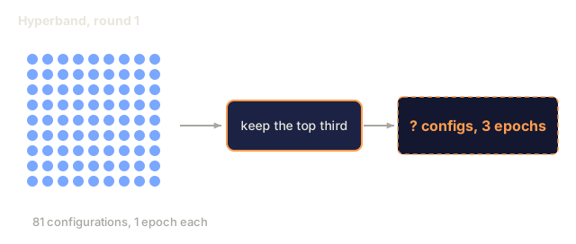
Hyperband is particularly effective. It starts 81 configurations with 1 epoch each, keeps the top third, gives them 3 epochs, keeps the top third, and so on. This finds good configurations 10-50x faster than evaluating all configs for the full budget.
Learning Rate Schedulers
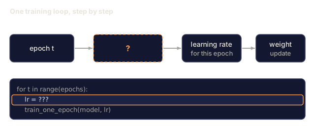
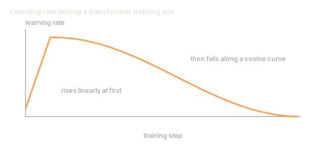
A learning rate scheduler adjusts the learning rate during training instead of holding it fixed. That matters because the learning rate is almost always the single most important hyperparameter you'll tune.
| Scheduler | Formula | When to use |
|---|---|---|
| Step decay | Multiply by 0.1 every N epochs | Classic CNN training |
| Cosine annealing | lr * 0.5 * (1 + cos(pi * t / T)) | Modern default |
| Warmup + decay | Linear increase then cosine decay | Transformers |
| One-cycle | Increase then decrease over one cycle | Fast convergence |
| Reduce on plateau | Reduce by factor when metric stalls | Safe default |
Hyperparameter Importance
Not all hyperparameters matter equally. Research on random forests (Probst et al., 2019) and gradient boosting shows consistent patterns:
High importance:
- Learning rate (always tune first)
- Number of estimators / epochs (use early stopping instead of tuning)
- Regularization strength
Medium importance:
- Max depth / number of layers
- Min samples per leaf / weight decay
- Subsample ratio
Low importance:
- Max features (for random forests)
- Specific activation function choice
- Batch size (within reasonable range)
Tune the important ones first, leave the rest at defaults.
Practical Strategy

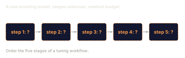
The concrete workflow:
- Start with library defaults. They are chosen by experienced practitioners and are often 80% of the way there.
- Coarse random search. Wide ranges, 20-50 trials. Use early stopping to kill bad runs fast.
- Analyze results. Which hyperparameters correlate with performance? Narrow the search space.
- Fine search. Bayesian optimization or focused random search in the narrowed space. 50-100 trials.
- Retrain on all training data with the best hyperparameters found.
Cross-Validation Integration
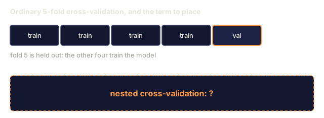
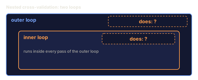
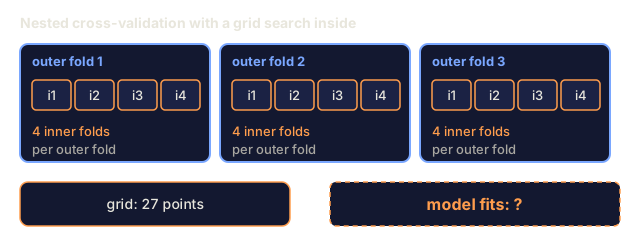
Nested cross-validation guards against a real risk: tuning hyperparameters against a single validation split can hand you hyperparameters that just overfit that one fold. It fixes this with two loops:
- Outer loop (evaluation): splits data into train+val and test. Reports unbiased performance.
- Inner loop (tuning): splits train+val into train and val. Finds best hyperparameters.

Each outer fold finds its own best hyperparameters independently. The outer scores are an unbiased estimate of generalization performance.
With sklearn:
from sklearn.model_selection import cross_val_score, GridSearchCV
from sklearn.ensemble import GradientBoostingRegressor

inner_cv = GridSearchCV(
    GradientBoostingRegressor(),
    param_grid={
        "learning_rate": [0.01, 0.05, 0.1],
        "max_depth": [2, 3, 5],
        "n_estimators": [50, 100, 200],
    },
    cv=5,
    scoring="neg_mean_squared_error",
)

outer_scores = cross_val_score(
    inner_cv, X, y, cv=5, scoring="neg_mean_squared_error"
)

print(f"Nested CV MSE: {-outer_scores.mean():.4f} +/- {outer_scores.std():.4f}")
This is expensive (5 outer folds x 5 inner folds x 27 grid points = 675 model fits), but it gives you a trustworthy performance estimate. Use it when reporting final results in papers, or when the stakes of the decision are high.
Practical Tips
Start with the learning rate. It is always the most important hyperparameter for gradient-based methods. A bad learning rate makes everything else irrelevant. Fix other hyperparameters at defaults and sweep learning rate first.
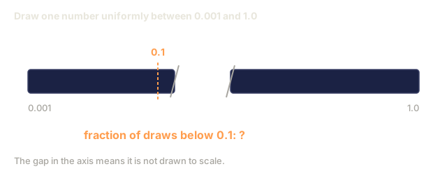
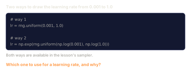
Use log-uniform distributions for learning rate and regularization. The difference between 0.001 and 0.01 matters as much as the difference between 0.1 and 1.0. Searching linearly wastes budget on the large end.
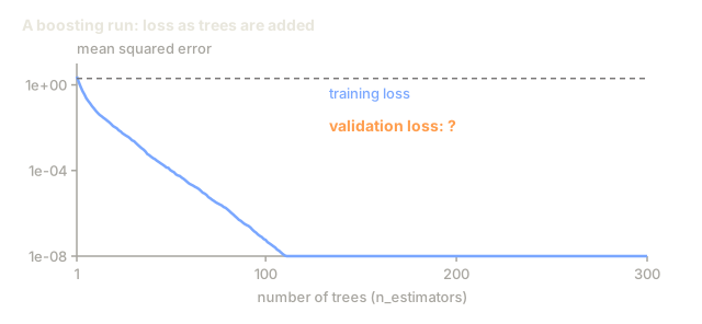
Use early stopping instead of tuning n_estimators. For boosting and neural networks, set n_estimators or epochs high and let early stopping decide when to stop. This removes one hyperparameter from the search.
Budget allocation. Put 60% of your tuning budget on the top 2 most important hyperparameters and the remaining 40% on everything else. Those top 2 account for most of the performance variation.
Scale matters. Never search batch size on a log scale (16, 32, 64 are fine). Always search learning rate on a log scale. Match the search distribution to how the hyperparameter affects the model.
| Model Type | Top Hyperparameters | Recommended Search | Budget |
|---|---|---|---|
| Random Forest | n_estimators, max_depth, min_samples_leaf | Random search, 50 trials | Low (fast training) |
| Gradient Boosting | learning_rate, n_estimators, max_depth | Bayesian, 100 trials + early stopping | Medium |
| Neural Network | learning_rate, weight_decay, batch_size | Bayesian or random, 100+ trials | High (slow training) |
| SVM | C, gamma (RBF kernel) | Grid on log scale, 25-50 trials | Low (2 params) |
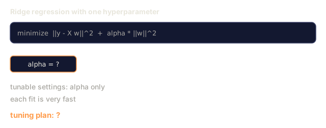
| Lasso/Ridge | alpha | 1D search on log scale, 20 trials | Very low |
| XGBoost | learning_rate, max_depth, subsample, colsample | Bayesian, 100-200 trials + early stopping | Medium |
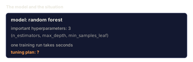
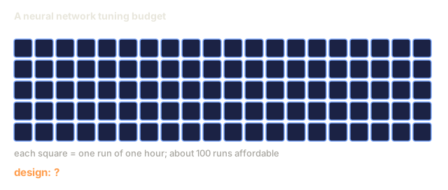
When in doubt: random search with 2x the number of hyperparameters as trials (e.g., 6 hyperparameters = 12+ trials minimum). Random search with just 50 trials beats a carefully designed grid search more often than it should.
Build It
Step 1: Grid Search from Scratch
The code in code/tuning.py implements grid search, random search, and a simple Bayesian optimizer from scratch.
def grid_search(model_fn, param_grid, X_train, y_train, X_val, y_val):
    keys = list(param_grid.keys())
    values = list(param_grid.values())
    best_score = -float("inf")
    best_params = None
    n_evals = 0

    for combo in itertools.product(*values):
        params = dict(zip(keys, combo))
        model = model_fn(**params)
        model.fit(X_train, y_train)
        score = evaluate(model, X_val, y_val)
        n_evals += 1

        if score > best_score:
            best_score = score
            best_params = params

    return best_params, best_score, n_evals
Step 2: Random Search from Scratch
def random_search(model_fn, param_distributions, X_train, y_train,
                  X_val, y_val, n_iter=50, seed=42):
    rng = np.random.RandomState(seed)
    best_score = -float("inf")
    best_params = None

    for _ in range(n_iter):
        params = {k: sample(v, rng) for k, v in param_distributions.items()}
        model = model_fn(**params)
        model.fit(X_train, y_train)
        score = evaluate(model, X_val, y_val)

        if score > best_score:
            best_score = score
            best_params = params

    return best_params, best_score, n_iter
Step 3: Bayesian Optimization (Simplified)
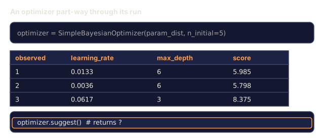
The core idea: fit a Gaussian process to observed (hyperparameter, score) pairs, then use an acquisition function to decide where to look next.
class SimpleBayesianOptimizer:
    def __init__(self, search_space, n_initial=5):
        self.search_space = search_space
        self.n_initial = n_initial
        self.X_observed = []
        self.y_observed = []

    def _kernel(self, x1, x2, length_scale=1.0):
        dists = np.sum((x1[:, None, :] - x2[None, :, :]) ** 2, axis=2)
        return np.exp(-0.5 * dists / length_scale ** 2)

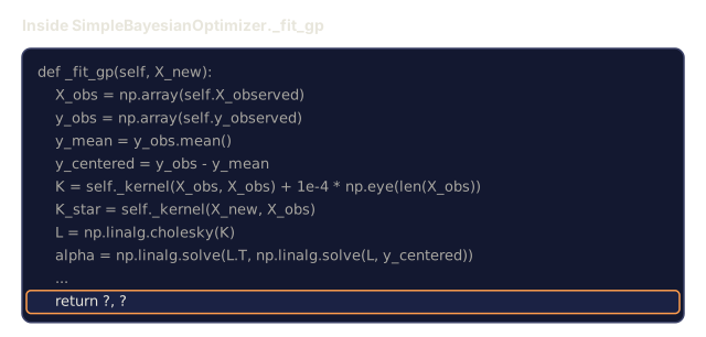
    def _fit_gp(self, X_new):
        X_obs = np.array(self.X_observed)
        y_obs = np.array(self.y_observed)
        y_mean = y_obs.mean()
        y_centered = y_obs - y_mean

        K = self._kernel(X_obs, X_obs) + 1e-4 * np.eye(len(X_obs))
        K_star = self._kernel(X_new, X_obs)

        L = np.linalg.cholesky(K)
        alpha = np.linalg.solve(L.T, np.linalg.solve(L, y_centered))
        mu = K_star @ alpha + y_mean

        v = np.linalg.solve(L, K_star.T)
        var = 1.0 - np.sum(v ** 2, axis=0)
        var = np.maximum(var, 1e-6)

        return mu, var

    def _expected_improvement(self, mu, var, best_y):
        sigma = np.sqrt(var)
        z = (mu - best_y) / (sigma + 1e-10)
        ei = sigma * (z * norm_cdf(z) + norm_pdf(z))
        return ei

    def suggest(self):
        if len(self.X_observed) < self.n_initial:
            return sample_random(self.search_space)

        candidates = [sample_random(self.search_space) for _ in range(500)]
        X_cand = np.array([to_vector(c) for c in candidates])
        mu, var = self._fit_gp(X_cand)
        ei = self._expected_improvement(mu, var, max(self.y_observed))
        return candidates[np.argmax(ei)]

    def observe(self, params, score):
        self.X_observed.append(to_vector(params))
        self.y_observed.append(score)
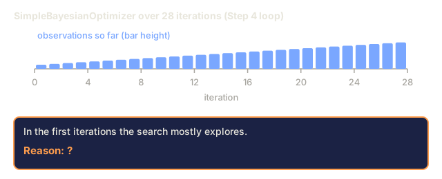
The GP surrogate gives two things at each candidate point: a predicted score (mu) and an uncertainty (var). Expected Improvement balances these: it favors points where the model predicts high scores OR where uncertainty is high. Early on, most points have high uncertainty so the optimizer explores. Later, it focuses on the most promising region.
Step 4: Compare All Methods
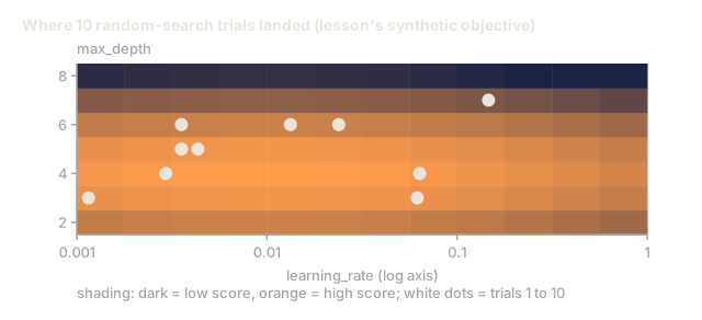
Run all three methods on the same synthetic objective and compare them directly. This version calls each optimizer against a plain objective function instead of training a model, so the API looks a little different from the model-based implementations above:
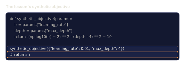
def synthetic_objective(params):
    lr = params["learning_rate"]
    depth = params["max_depth"]
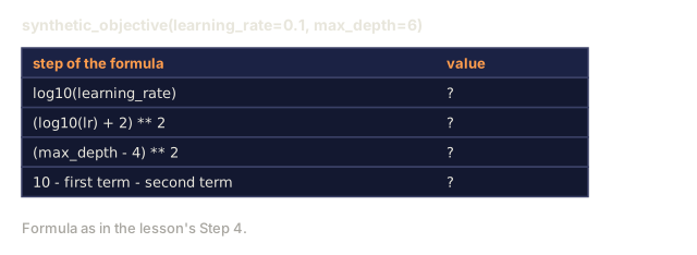
    return -(np.log10(lr) + 2) ** 2 - (depth - 4) ** 2 + 10

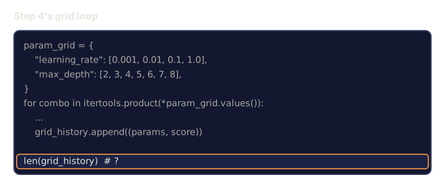
param_grid = {
    "learning_rate": [0.001, 0.01, 0.1, 1.0],
    "max_depth": [2, 3, 4, 5, 6, 7, 8],
}

grid_best = None
grid_score = -float("inf")
grid_history = []
for combo in itertools.product(*param_grid.values()):
    params = dict(zip(param_grid.keys(), combo))
    score = synthetic_objective(params)
    grid_history.append((params, score))
    if score > grid_score:
        grid_score = score
        grid_best = params

param_dist = {
    "learning_rate": ("log_float", 0.001, 1.0),
    "max_depth": ("int", 2, 8),
}

rand_best = None
rand_score = -float("inf")
rand_history = []
rng = np.random.RandomState(42)
for _ in range(28):
    params = {k: sample(v, rng) for k, v in param_dist.items()}
    score = synthetic_objective(params)
    rand_history.append((params, score))
    if score > rand_score:
        rand_score = score
        rand_best = params

optimizer = SimpleBayesianOptimizer(param_dist, n_initial=5)
bayes_history = []
for _ in range(28):
    params = optimizer.suggest()
    score = synthetic_objective(params)
    optimizer.observe(params, score)
    bayes_history.append((params, score))
bayes_score = max(s for _, s in bayes_history)

print(f"{'Method':<20} {'Best Score':>12} {'Evaluations':>12}")
print("-" * 50)
print(f"{'Grid Search':<20} {grid_score:>12.4f} {len(grid_history):>12}")
print(f"{'Random Search':<20} {rand_score:>12.4f} {len(rand_history):>12}")
print(f"{'Bayesian Opt':<20} {bayes_score:>12.4f} {len(bayes_history):>12}")
With the same budget, Bayesian optimization usually finds the best score fastest because it does not waste evaluations in clearly bad regions. Random search covers more ground than grid search. Grid search only wins when you have very few hyperparameters and can afford to be exhaustive.
Use It
Optuna in Practice
Optuna is the recommended library for serious hyperparameter tuning. It supports pruning, distributed search, and visualization out of the box.
import optuna

def objective(trial):
    lr = trial.suggest_float("learning_rate", 1e-4, 1e-1, log=True)
    n_est = trial.suggest_int("n_estimators", 50, 500)
    max_depth = trial.suggest_int("max_depth", 2, 10)

    model = GradientBoostingRegressor(
        learning_rate=lr,
        n_estimators=n_est,
        max_depth=max_depth,
    )
    model.fit(X_train, y_train)
    return mean_squared_error(y_val, model.predict(X_val))

study = optuna.create_study(direction="minimize")
study.optimize(objective, n_trials=100)

print(f"Best params: {study.best_params}")
print(f"Best MSE: {study.best_value:.4f}")
Key Optuna features:
suggest_float(..., log=True)for parameters best searched on log scale (learning rate, regularization)suggest_intfor integer parameterssuggest_categoricalfor discrete choices- Built-in MedianPruner for early stopping of bad trials
study.trials_dataframe()for analysis
Optuna with Pruning
Pruning stops unpromising trials early, saving massive compute. Here is the pattern:
import optuna
from sklearn.model_selection import cross_val_score

def objective(trial):
    params = {
        "learning_rate": trial.suggest_float("lr", 1e-4, 0.5, log=True),
        "max_depth": trial.suggest_int("max_depth", 2, 10),
        "n_estimators": trial.suggest_int("n_estimators", 50, 500),
        "subsample": trial.suggest_float("subsample", 0.5, 1.0),
    }

    model = GradientBoostingRegressor(**params)
    scores = cross_val_score(model, X_train, y_train, cv=3,
                             scoring="neg_mean_squared_error")
    mean_score = -scores.mean()

    trial.report(mean_score, step=0)
    if trial.should_prune():
        raise optuna.TrialPruned()

    return mean_score

pruner = optuna.pruners.MedianPruner(n_startup_trials=10, n_warmup_steps=5)
study = optuna.create_study(direction="minimize", pruner=pruner)
study.optimize(objective, n_trials=200)
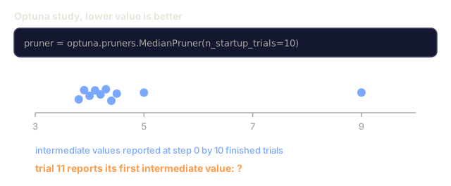
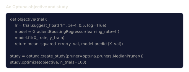
The MedianPruner stops a trial if its intermediate value is worse than the median of all completed trials at the same step. Pruning requires calling trial.report() to report intermediate metrics and trial.should_prune() to check whether the trial should be stopped. The n_startup_trials=10 ensures at least 10 trials complete fully before pruning kicks in. This typically saves 40-60% of total compute.
sklearn's Built-in Tuners
For quick experiments, sklearn provides GridSearchCV, RandomizedSearchCV, and HalvingRandomSearchCV:
from sklearn.model_selection import RandomizedSearchCV
from scipy.stats import loguniform, randint

param_dist = {
    "learning_rate": loguniform(1e-4, 0.5),
    "max_depth": randint(2, 10),
    "n_estimators": randint(50, 500),
}

search = RandomizedSearchCV(
    GradientBoostingRegressor(),
    param_dist,
    n_iter=100,
    cv=5,
    scoring="neg_mean_squared_error",
    random_state=42,
    n_jobs=-1,
)
search.fit(X_train, y_train)
print(f"Best params: {search.best_params_}")
print(f"Best CV MSE: {-search.best_score_:.4f}")
Use loguniform from scipy for learning rate and regularization. Use randint for integer hyperparameters. The n_jobs=-1 flag parallelizes across all CPU cores.
Common Mistakes in Hyperparameter Tuning
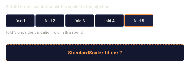
Data leakage through preprocessing. If you fit a scaler on the full dataset before cross-validation, information from the validation fold leaks into training. Always put preprocessing inside a Pipeline so it is fit only on the training fold.
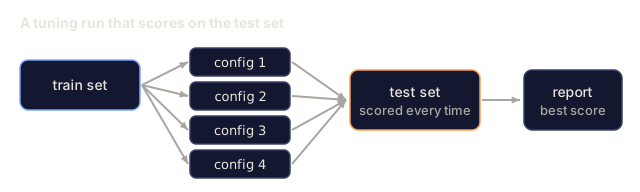
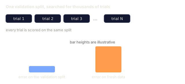
Overfitting to the validation set. Running thousands of trials effectively trains on the validation set. Use nested cross-validation for final performance estimates, or hold out a separate test set that you never touch during tuning.
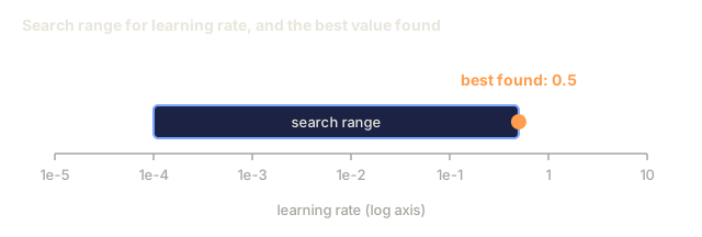
Searching too narrow a range. If your best value sits at the boundary of your search space, the true optimum is probably outside it. Check whether the best parameters land at the edges before you trust the result.
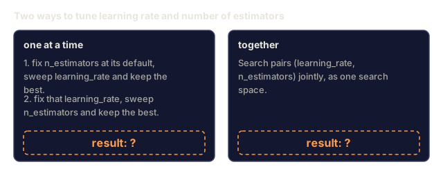
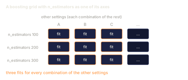
Ignoring interaction effects. Learning rate and number of estimators interact strongly in boosting. A low learning rate needs more estimators. Tuning them independently gives worse results than tuning them together.
Not using early stopping for iterative models. For gradient boosting and neural networks, set n_estimators or epochs to a high value and use early stopping. This is strictly better than tuning the number of iterations as a hyperparameter.
The tool people reach for first is almost always the wrong one for their problem. I've watched teams spend a week wiring up Optuna with a Gaussian process pruner to tune a random forest that trains in four seconds, when fifty lines of random search would have found the same answer before the Optuna config was even finished. Bayesian optimization earns its overhead when training itself is expensive: an hour per run, a GPU cluster, a search space nobody has mapped before. Below that, it's just extra machinery.
The mistake that actually burns money is a different one: tuning n_estimators or epochs by hand instead of turning on early stopping. I still see grid search running over number of trees in production pipelines, paying for compute the model would have told you to stop spending if you'd just let validation loss flatten out on its own. Fix that habit before you touch anything fancier.
Exercises
-
Run grid search and random search with the same total budget (e.g., 50 evaluations). Compare the best scores found. Run the experiment 10 times with different seeds. How often does random search win?
-
Implement Hyperband from scratch. Start with 81 configurations, each trained for 1 epoch. Keep the top 1/3 at each round and triple their budget. Compare total compute (sum of all epochs across all configs) to running 81 configs for the full budget.
-
Add a learning rate scheduler (cosine annealing) to the gradient boosting implementation from Lesson 11. Does it help compared to a fixed learning rate?
-
Use Optuna to tune a RandomForestClassifier on a real dataset (e.g., sklearn's breast cancer dataset). Use
optuna.visualization.plot_param_importances(study)to see which hyperparameters matter most. Does it match the importance ranking from this lesson? -
Implement a simple acquisition function (Expected Improvement) and demonstrate exploration vs exploitation. Plot the surrogate model's mean and uncertainty, and show where EI chooses to evaluate next.
Key Terms
| Term | What people say | What it actually means |
|---|---|---|
| Hyperparameter | "A setting you choose" | A value set before training that controls the learning process, not learned from data |
| Grid search | "Try every combination" | Exhaustive search over a specified parameter grid. Exponential cost. |
| Random search | "Just sample randomly" | Sample hyperparameters from distributions. Covers important dimensions better than grid search. |
| Bayesian optimization | "Smart search" | Uses a surrogate model of the objective to decide where to evaluate next, balancing exploration and exploitation |
| Surrogate model | "A cheap approximation" | A model (usually Gaussian process) that approximates the expensive objective function from observed evaluations |
| Acquisition function | "Where to look next" | Scores candidate points by balancing expected improvement with uncertainty. EI and UCB are common choices. |
| Early stopping | "Stop wasting time" | Terminate training early when validation performance stops improving |
| Hyperband | "Tournament bracket for configs" | Adaptive resource allocation: start many configs with small budgets, keep the best and increase their budgets |
| Learning rate scheduler | "Change lr during training" | A function that adjusts the learning rate over the course of training for better convergence |
Further Reading
- Bergstra & Bengio: Random Search for Hyper-Parameter Optimization (2012) -- the paper that showed random beats grid
- Snoek et al., Practical Bayesian Optimization of Machine Learning Algorithms (2012) -- Bayesian optimization for ML
- Li et al., Hyperband: A Novel Bandit-Based Approach (2018) -- the Hyperband paper
- Optuna: A Next-generation Hyperparameter Optimization Framework -- the Optuna paper
- Probst et al., Tunability: Importance of Hyperparameters (2019) -- which hyperparameters matter
Code
- tuning.py (python, 573 lines)