Introduction to JAX
PyTorch mutates tensors. TensorFlow builds graphs. JAX compiles pure functions. That last one changes how you think about deep learning.
Learning Objectives
- Write pure-function neural network code using JAX's functional API (jax.numpy, jax.grad, jax.jit, jax.vmap)
- Explain the key design difference between PyTorch's eager mutation and JAX's functional compilation model
- Apply jit compilation and vmap vectorization to accelerate training loops compared to naive Python
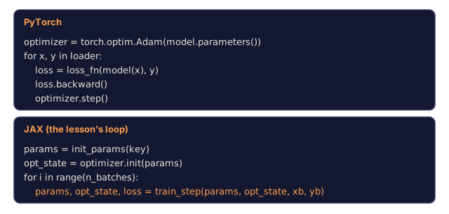
- Train a simple network in JAX and contrast the explicit state management with PyTorch's object-oriented approach
The Problem
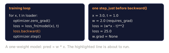
You know how to build neural networks in PyTorch. Define an nn.Module, call .backward(), step the optimizer. It works, and millions of people use it every day.
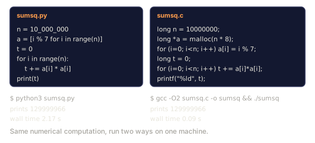
But PyTorch has a real constraint: it traces operations eagerly, one at a time, in Python. Every tensor + tensor is a separate kernel launch, and every training step re-interprets the same Python code. That's fine at normal scale. It stops being fine the moment you need to train a 540-billion-parameter model across 2,048 TPUs, where the overhead compounds into real time and real money.
JAX is NumPy with three superpowers: automatic differentiation, JIT compilation to XLA, and automatic vectorization. Write a function that processes one example, and JAX hands you back a function that processes a batch, computes gradients, compiles to machine code, and runs across multiple devices, all without touching the original function.
Google DeepMind trains Gemini on JAX. Anthropic trained Claude on JAX. These aren't small operations: they're the largest neural network training runs on Earth, and both labs chose JAX because it treats a training loop as a compilable program rather than a sequence of Python calls.
The Concept
The JAX Philosophy
JAX is a functional framework: no classes, no mutable state, no .backward() method. Instead:
| PyTorch | JAX |
|---|---|
nn.Module class with state | Pure function: f(params, x) -> y |
loss.backward() | jax.grad(loss_fn)(params, x, y) |
| Eager execution | JIT compilation via XLA |
for x in batch: manual loop | jax.vmap(f) auto-vectorization |
DataParallel / FSDP (PyTorch's multi-GPU wrappers) | jax.pmap(f) auto-parallelism |
Mutable model.parameters() | Immutable pytree of arrays |
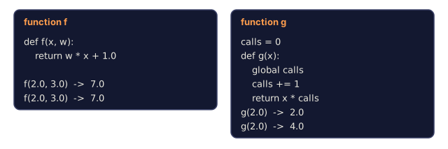
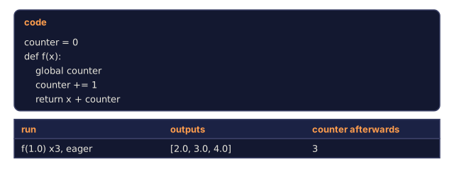
This isn't a style preference, it's a compiler constraint. JIT compilation requires pure functions: the same inputs always produce the same outputs, with no side effects. That restriction is exactly what makes 100x speedups possible.
jax.numpy: The Familiar Surface
JAX reimplements the NumPy API on accelerators:
import jax.numpy as jnp

a = jnp.array([1.0, 2.0, 3.0])
b = jnp.array([4.0, 5.0, 6.0])
c = jnp.dot(a, b)
Same function names, same broadcasting rules, same slicing semantics. The difference is that these arrays live on GPU or TPU, and every operation is traceable by the compiler.
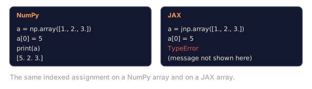
One critical difference: JAX arrays are immutable. There's no a[0] = 5, only a = a.at[0].set(5). It feels awkward for about a week. Then it clicks: immutability is exactly what makes transformations like grad, jit, and vmap composable.
jax.grad: Functional Autodiff
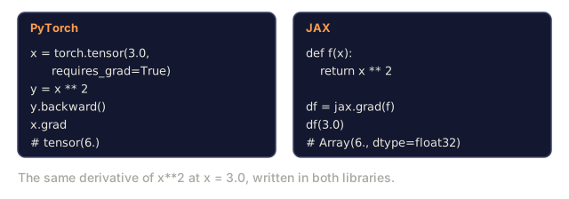
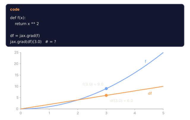
jax.grad takes a function and returns a new function that computes its gradient. PyTorch attaches gradients to tensors (.grad); JAX attaches them to functions instead:
import jax

def f(x):
    return x ** 2

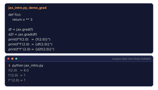
df = jax.grad(f)
df(3.0)
There's no .backward() call and no computation graph stored on tensors. The gradient is just another function you can call, compose, or JIT-compile.
This composes arbitrarily:
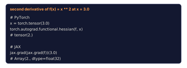
d2f = jax.grad(jax.grad(f))
d2f(3.0)
Second derivatives, third derivatives, Jacobians, Hessians: all of it by composing grad. PyTorch can do this too, through torch.autograd.functional.hessian, but it's bolted on. In JAX, composable grad is the foundation.
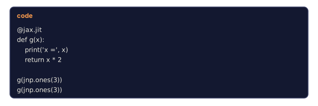
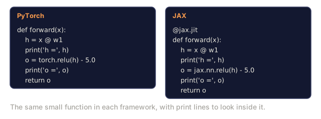
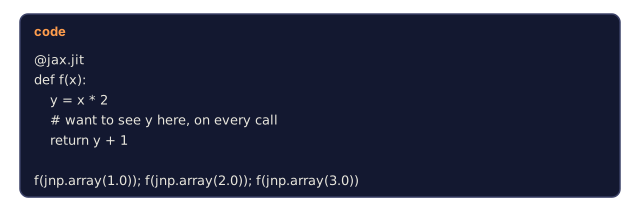
The constraint: grad only works on pure functions. No print statements inside, since they run during tracing rather than execution, no mutation of external state, and no random number generation without explicit key management.
jit: Compile to XLA
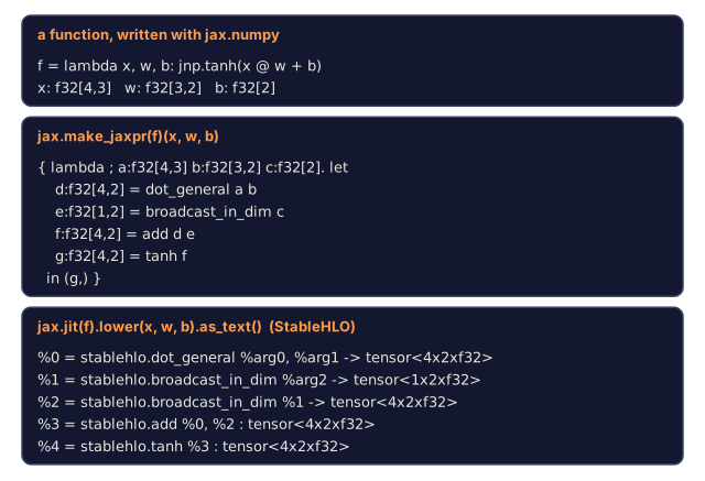
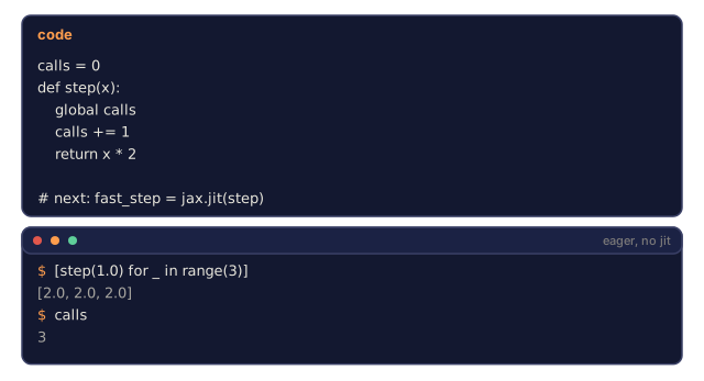
jax.jit traces a function once, hands that trace to XLA, and swaps in the compiled version for every call after:
@jax.jit
def train_step(params, x, y):
    loss = loss_fn(params, x, y)
    return loss

fast_step = jax.jit(train_step)
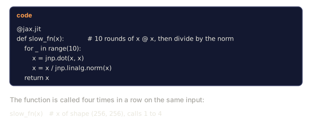
On the first call, JAX traces the function: it records which operations happen without executing them. Then it hands that trace to XLA (Accelerated Linear Algebra), Google's compiler for TPUs and GPUs. XLA fuses operations, eliminates redundant memory copies, and generates optimized machine code.
Subsequent calls skip Python entirely. The compiled code runs on the accelerator at C++ speed.
When JIT helps:
- Training steps (same computation repeated thousands of times)
- Inference (same model, different inputs)
- Any function called more than once with similar-shaped inputs
When JIT hurts:
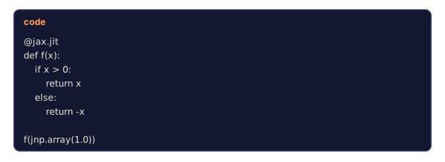
- Functions with Python control flow that depends on values (
if x > 0where x is a traced array) - One-shot computations, where compilation overhead exceeds runtime
- Debugging, since tracing hides the actual execution
The control flow restriction is real. jax.lax.cond replaces if/else, and jax.lax.scan replaces for loops. Neither is optional. They're the price of compilation.
vmap: Automatic Vectorization
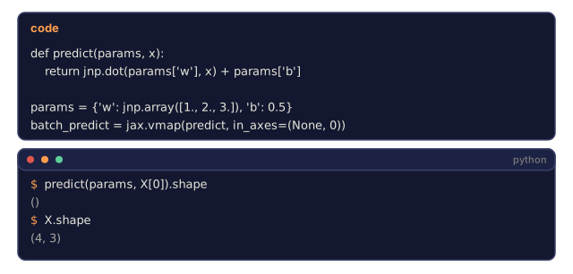
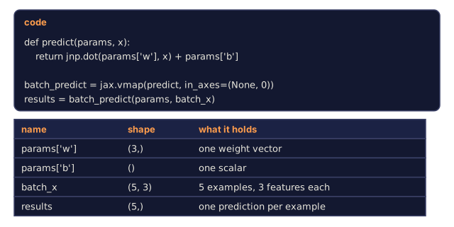
Write a function that processes one example:
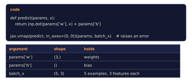
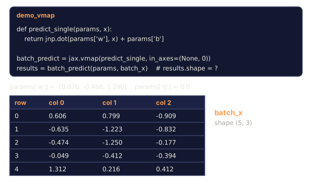
def predict(params, x):
    return jnp.dot(params['w'], x) + params['b']
vmap lifts it to process a batch:
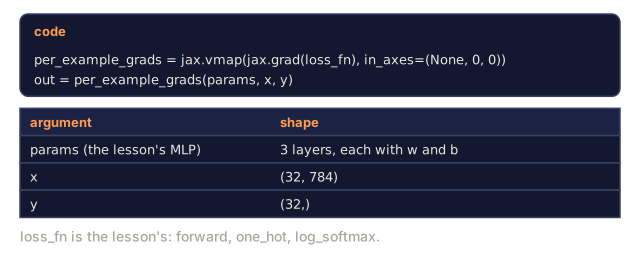
batch_predict = jax.vmap(predict, in_axes=(None, 0))in_axes=(None, 0) means don't batch over params, since it's shared, but do batch over axis 0 of x. There's no manual for loop, no reshaping, no batch dimension threading by hand. JAX figures out the batch dimension itself and vectorizes the entire computation.
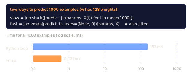
This isn't syntactic sugar. vmap generates fused vectorized code that runs 10-100x faster than a Python loop, and it composes with jit and grad:
per_example_grads = jax.vmap(jax.grad(loss_fn), in_axes=(None, 0, 0))Per-example gradients, in one line, something that's nearly impossible in PyTorch without hacks.
pmap: Data Parallelism Across Devices
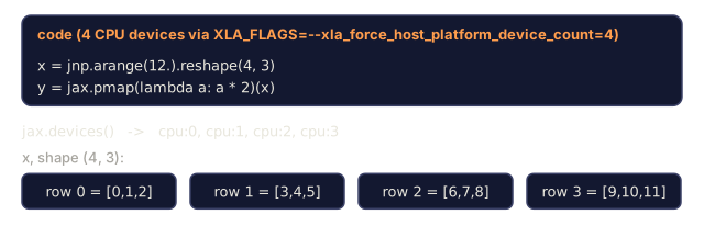
pmap replicates a function across every available device, GPUs or TPUs, and splits the batch between them:
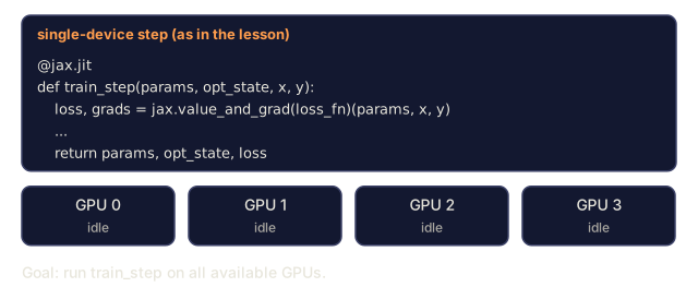
parallel_step = jax.pmap(train_step, axis_name='devices')Inside the function, jax.lax.pmean and jax.lax.psum synchronize gradients across devices. Google trains Gemini across thousands of TPU v5e chips this way, using pmap and its successor shard_map. The whole programming model comes down to: write the single-device version, wrap it with pmap, done.
Pytrees: The Universal Data Structure
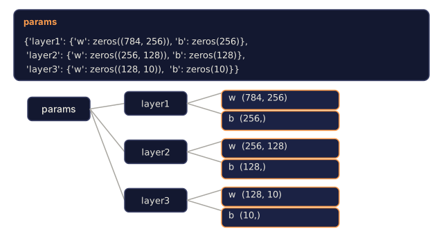
JAX operates on "pytrees": nested combinations of lists, tuples, dicts, and arrays. Your model parameters are a pytree:
params = {
    'layer1': {'w': jnp.zeros((784, 256)), 'b': jnp.zeros(256)},
    'layer2': {'w': jnp.zeros((256, 128)), 'b': jnp.zeros(128)},
    'layer3': {'w': jnp.zeros((128, 10)),  'b': jnp.zeros(10)},
}
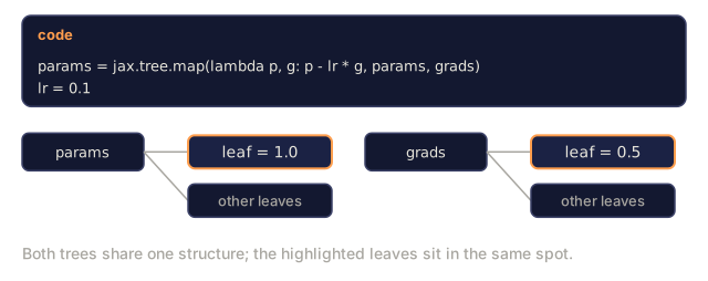
Every JAX transformation, grad, jit, vmap, knows how to traverse pytrees. jax.tree.map(f, tree) applies f to every leaf, which is how optimizers update all parameters at once:
params = jax.tree.map(lambda p, g: p - lr * g, params, grads)There's no .parameters() method and no parameter registration. The tree structure is the model.
Functional vs Object-Oriented
PyTorch stores state inside objects:
class Model(nn.Module):
    def __init__(self):
        self.linear = nn.Linear(784, 10)

    def forward(self, x):
        return self.linear(x)
JAX uses pure functions with explicit state instead:
def predict(params, x):
    return jnp.dot(x, params['w']) + params['b']
The params are passed in, nothing is stored, and nothing is mutated. That's what makes every function testable, composable, and compilable. It also means you're on the hook for managing the params yourself, or you reach for a library like Flax or Equinox.
The JAX Ecosystem
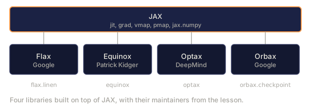
JAX gives you the primitives; libraries give you the ergonomics:
| Library | Role | Style |
|---|---|---|
| Flax (Google) | Neural network layers | nn.Module with explicit state |
| Equinox (Patrick Kidger) | Neural network layers | Pytree-based, Pythonic |
| Optax (DeepMind) | Optimizers + LR schedules | Composable gradient transforms |
| Orbax (Google) | Checkpointing | Save/restore pytrees |
| CLU (Google) | Metrics + logging | Training loop utilities |
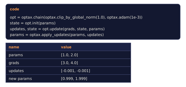
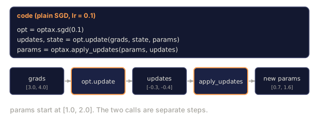
Optax is the standard optimizer library. It separates the gradient transformation (Adam, SGD, clipping) from the parameter update, which makes the two trivial to compose:
optimizer = optax.chain(
    optax.clip_by_global_norm(1.0),
    optax.adam(learning_rate=1e-3),
)
When to Use JAX vs PyTorch
| Factor | JAX | PyTorch |
|---|---|---|
| TPU support | First-class (Google built both) | Community-maintained (torch_xla) |
| GPU support | Good (CUDA via XLA) | Best-in-class (native CUDA) |
| Debugging | Hard (tracing + compilation) | Easy (eager, line-by-line) |
| Ecosystem | Research-focused (Flax, Equinox) | Massive (HuggingFace, torchvision, etc.) |
| Hiring | Niche (Google/DeepMind/Anthropic) | Mainstream (everywhere) |
| Large-scale training | Superior (XLA, pmap, mesh) | Good (FSDP, DeepSpeed) |
| Prototyping speed | Slower (functional overhead) | Faster (mutate and go) |
| Production inference | TensorFlow Serving, Vertex AI | TorchServe, Triton, ONNX |
| Who uses it | DeepMind (Gemini), Anthropic (Claude) | Meta (Llama), OpenAI (GPT), Stability AI |
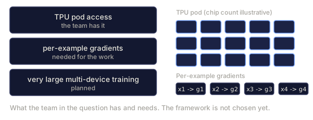
The honest answer: use PyTorch unless you have a specific reason to reach for JAX instead. Those reasons are narrow: TPU access, a real need for per-example gradients, multi-device training at massive scale, or working somewhere like Google, DeepMind, or Anthropic.
Random Numbers in JAX
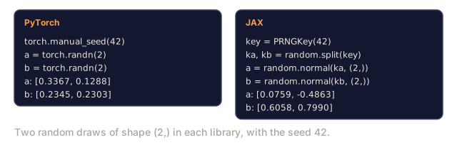
JAX has no global random state. Every random operation requires an explicit PRNG key:
key = jax.random.PRNGKey(42)
key1, key2 = jax.random.split(key)
w = jax.random.normal(key1, shape=(784, 256))
It's annoying at first, but it buys you something real: reproducibility across devices and compilations, a guarantee PyTorch's torch.manual_seed can't make in multi-GPU settings.
Build It
Step 1: Setup and Data
We'll train a 3-layer MLP on MNIST using JAX and Optax: 784 inputs, two hidden layers of 256 and 128 neurons, 10 output classes.
import jax
import jax.numpy as jnp
from jax import random
import optax

def get_mnist_data():
    from sklearn.datasets import fetch_openml
    mnist = fetch_openml('mnist_784', version=1, as_frame=False, parser='auto')
    X = mnist.data.astype('float32') / 255.0
    y = mnist.target.astype('int')
    X_train, X_test = X[:60000], X[60000:]
    y_train, y_test = y[:60000], y[60000:]
    return X_train, y_train, X_test, y_test
Step 2: Initialize Parameters
No class, just a function that returns a pytree:
def init_params(key):
    k1, k2, k3 = random.split(key, 3)
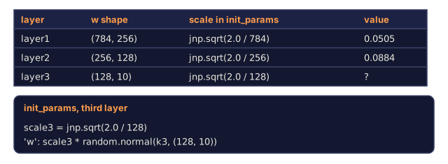
    scale1 = jnp.sqrt(2.0 / 784)
    scale2 = jnp.sqrt(2.0 / 256)
    scale3 = jnp.sqrt(2.0 / 128)
    params = {
        'layer1': {
            'w': scale1 * random.normal(k1, (784, 256)),
            'b': jnp.zeros(256),
        },
        'layer2': {
            'w': scale2 * random.normal(k2, (256, 128)),
            'b': jnp.zeros(128),
        },
        'layer3': {
            'w': scale3 * random.normal(k3, (128, 10)),
            'b': jnp.zeros(10),
        },
    }
    return params
This is He-initialization done by hand: three PRNG keys split from one seed, and every weight stored as an immutable array in a nested dict.
Step 3: Forward Pass
def forward(params, x):
    x = jnp.dot(x, params['layer1']['w']) + params['layer1']['b']
    x = jax.nn.relu(x)
    x = jnp.dot(x, params['layer2']['w']) + params['layer2']['b']
    x = jax.nn.relu(x)
    x = jnp.dot(x, params['layer3']['w']) + params['layer3']['b']
    return x

def loss_fn(params, x, y):
    logits = forward(params, x)
    one_hot = jax.nn.one_hot(y, 10)
    return -jnp.mean(jnp.sum(jax.nn.log_softmax(logits) * one_hot, axis=-1))
These are pure functions: params in, prediction out, no self, no stored state. loss_fn computes cross-entropy from scratch: softmax, log, negative mean.
Step 4: JIT-Compiled Training Step
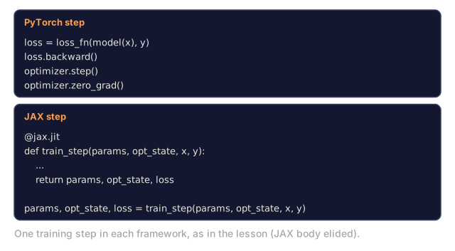
@jax.jit
def train_step(params, opt_state, x, y):
    loss, grads = jax.value_and_grad(loss_fn)(params, x, y)
    updates, opt_state = optimizer.update(grads, opt_state, params)
    params = optax.apply_updates(params, updates)
    return params, opt_state, loss

@jax.jit
def accuracy(params, x, y):
    logits = forward(params, x)
    preds = jnp.argmax(logits, axis=-1)
    return jnp.mean(preds == y)
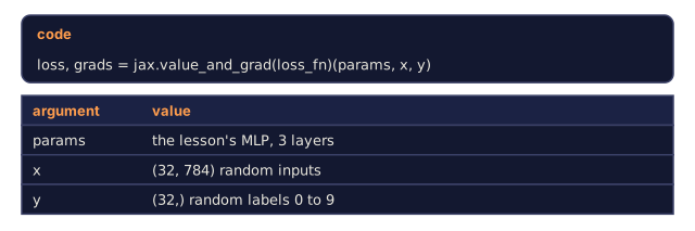
jax.value_and_grad returns the loss value and the gradients in a single pass. The @jax.jit decorator compiles both functions to XLA, so after the first call, every training step runs without touching Python again.
Step 5: Training Loop
optimizer = optax.adam(learning_rate=1e-3)

X_train, y_train, X_test, y_test = get_mnist_data()
X_train, X_test = jnp.array(X_train), jnp.array(X_test)
y_train, y_test = jnp.array(y_train), jnp.array(y_test)

key = random.PRNGKey(0)
params = init_params(key)
opt_state = optimizer.init(params)

batch_size = 128
n_epochs = 10

for epoch in range(n_epochs):
    key, subkey = random.split(key)
    perm = random.permutation(subkey, len(X_train))
    X_shuffled = X_train[perm]
    y_shuffled = y_train[perm]

    epoch_loss = 0.0
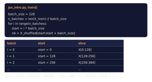
    n_batches = len(X_train) // batch_size
    for i in range(n_batches):
        start = i * batch_size
        xb = X_shuffled[start:start + batch_size]
        yb = y_shuffled[start:start + batch_size]
        params, opt_state, loss = train_step(params, opt_state, xb, yb)
        epoch_loss += loss

    train_acc = accuracy(params, X_train[:5000], y_train[:5000])
    test_acc = accuracy(params, X_test, y_test)
    print(f"Epoch {epoch + 1:2d} | Loss: {epoch_loss / n_batches:.4f} | "
          f"Train Acc: {train_acc:.4f} | Test Acc: {test_acc:.4f}")
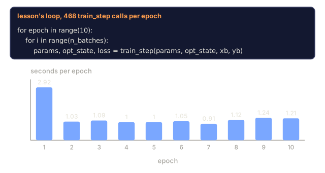
Ten epochs gets you roughly 97% test accuracy. The first epoch is slow because of JIT compilation; epochs 2 through 10 run fast.
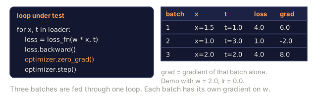
Notice what's missing: no .zero_grad(), no .backward(), no .step(). The entire update is one composed function call, with gradients computed, transformed by Adam, and applied to parameters, all inside train_step.
Use It
Flax: The Google Standard
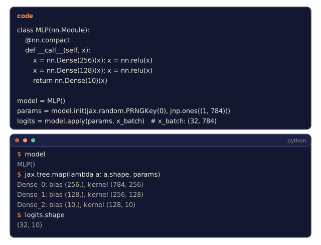
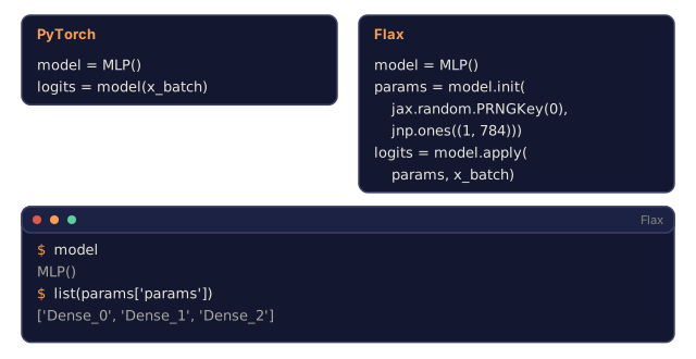
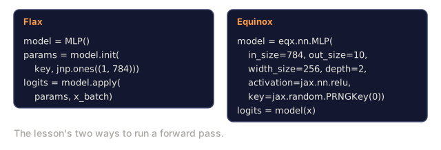
Flax is the most common JAX neural network library. It adds nn.Module back, but with explicit state management:
import flax.linen as nn

class MLP(nn.Module):
    @nn.compact
    def __call__(self, x):
        x = nn.Dense(256)(x)
        x = nn.relu(x)
        x = nn.Dense(128)(x)
        x = nn.relu(x)
        x = nn.Dense(10)(x)
        return x

model = MLP()
params = model.init(jax.random.PRNGKey(0), jnp.ones((1, 784)))
logits = model.apply(params, x_batch)
The structure looks like PyTorch, but params lives separately from the model: model.init() creates the params, model.apply(params, x) runs the forward pass, and the model object itself holds no state.
Equinox: The Pythonic Alternative
Equinox (by Patrick Kidger) represents models as pytrees:
import equinox as eqx

model = eqx.nn.MLP(
    in_size=784, out_size=10, width_size=256, depth=2,
    activation=jax.nn.relu, key=jax.random.PRNGKey(0)
)
logits = model(x)
The model itself is a pytree, so there's no .apply() needed. Parameters are just the model's leaves, which is closer to how JAX actually thinks.
Optax: Composable Optimizers
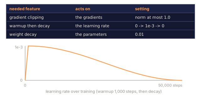
Optax decouples the gradient transformation from the update:
schedule = optax.warmup_cosine_decay_schedule(
    init_value=0.0, peak_value=1e-3,
    warmup_steps=1000, decay_steps=50000
)

optimizer = optax.chain(
    optax.clip_by_global_norm(1.0),
    optax.adamw(learning_rate=schedule, weight_decay=0.01),
)
Gradient clipping, learning rate warmup, and weight decay all compose as a chain of transforms: each one sees the gradients, modifies them, and passes them to the next, with no monolithic optimizer class in sight.
Ship It
Installation:
pip install jax jaxlib optax flaxFor GPU support:
pip install jax[cuda12]For TPU (Google Cloud):
pip install jax[tpu] -f https://storage.googleapis.com/jax-releases/libtpu_releases.htmlPerformance gotchas:
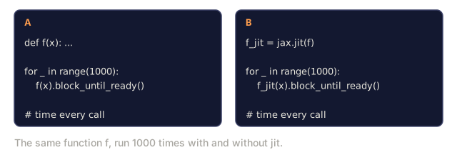
- First JIT call is slow (compilation). Warm up before benchmarking.
- Avoid Python loops over JAX arrays inside JIT. Use
jax.lax.scanorjax.lax.fori_loop. jax.debug.print()works inside JIT. Regularprint()does not.- Profile with
jax.profileror TensorBoard. XLA compilation can hide bottlenecks. - JAX pre-allocates 75% of GPU memory by default. Set
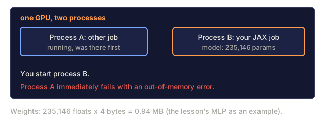
XLA_PYTHON_CLIENT_PREALLOCATE=falseto disable.
Checkpointing:
import orbax.checkpoint as ocp
checkpointer = ocp.PyTreeCheckpointer()
checkpointer.save('/tmp/model', params)
restored = checkpointer.restore('/tmp/model')
This lesson produces:
outputs/prompt-jax-optimizer.md: a prompt for choosing the right JAX optimizer configurationoutputs/skill-jax-patterns.md: a skill covering functional patterns in JAX
Most people who work through this lesson will never touch JAX again day to day, and that's fine. Unless you're training at Google scale or need per-example gradients for something like differential privacy, PyTorch is still the right default. I said that above and I mean it.
What's worth keeping even if you never import jax again is the discipline underneath it: write your training step as a pure function first, figure out what state it actually needs, then decide how to manage that state, explicitly and on purpose, instead of letting a base class hand it to you. That habit alone makes PyTorch code easier to debug, because you stop discovering mutations three functions away that you never meant to happen.
One more thing: don't judge JAX by how it feels in week one. The immutable arrays and the explicit PRNG keys read like friction right up until the moment you need to reproduce a bug across two GPUs and torch.manual_seed won't get you there. That's usually the week it clicks.
Exercises
-
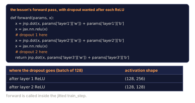
Add dropout to the MLP. In JAX, dropout requires a PRNG key: thread a key through the forward pass and split it for each dropout layer, then compare test accuracy with and without.
-
Use
jax.vmapto compute per-example gradients for a batch of 32 MNIST images. Compute the gradient norm for each example. Which examples have the largest gradients, and why? -
Replace the manual forward function with a generic
mlp_forward(params, x)that works for any number of layers. Usejax.tree.leavesto determine the depth automatically. -
Benchmark the training step with and without
@jax.jit. Time 100 steps of each. How large is the speedup on your hardware? What is the compilation overhead on the first call? -
Implement gradient clipping by composing
optax.chain(optax.clip_by_global_norm(1.0), optax.adam(1e-3)). Train with and without clipping. Plot the gradient norm over training to see the effect.
Key Terms
| Term | What people say | What it actually means |
|---|---|---|
| XLA | "The thing that makes JAX fast" | Accelerated Linear Algebra: a compiler that fuses operations and generates optimized GPU/TPU kernels from a computation graph |
| JIT | "Just-in-time compilation" | JAX traces the function on first call, compiles to XLA, then runs the compiled version on subsequent calls |
| Pure function | "No side effects" | A function where the output depends only on inputs: no global state, no mutation, no randomness without explicit keys |
| vmap | "Auto-batching" | Transforms a function that processes one example into one that processes a batch, without rewriting |
| pmap | "Auto-parallelism" | Replicates a function across multiple devices and splits the input batch |
| Pytree | "Nested dict of arrays" | Any nested structure of lists, tuples, dicts, and arrays that JAX can traverse and transform |
| Tracing | "Recording the computation" | JAX executes the function with abstract values to build a computation graph, without computing real results |
| Functional autodiff | "grad of a function" | Computing derivatives by transforming functions, not by attaching gradient storage to tensors |
| Optax | "JAX's optimizer library" | A composable library of gradient transformations (Adam, SGD, clipping, scheduling) that chain together |
| Flax | "JAX's nn.Module" | Google's neural network library for JAX, adding layer abstractions while keeping state explicit |
Further Reading
- JAX documentation: https://jax.readthedocs.io/, the official docs, with excellent tutorials on grad, jit, and vmap
- "JAX: composable transformations of Python+NumPy programs" (Bradbury et al., 2018), the original paper explaining the design philosophy
- Flax documentation: https://flax.readthedocs.io/, Google's neural network library for JAX
- Patrick Kidger, "Equinox: neural networks in JAX via callable PyTrees and filtered transformations" (2021), the Pythonic alternative to Flax
- DeepMind, "Optax: composable gradient transformation and optimisation", the standard optimizer library
- "You Don't Know JAX" (Colin Raffel, 2020), a practical guide to JAX gotchas and patterns, from one of the T5 authors
Code
- jax_intro.py (python, 180 lines)