Spectrograms, Mel Scale & Audio Features
Neural nets barely tolerate raw waveforms. Hand them a spectrogram and they get traction; hand them a mel spectrogram and they get good. Every ASR, TTS, and audio classifier in 2026 lives or dies by that one preprocessing choice.
Learning Objectives
- Explain why raw waveforms are a poor model input and how the STFT turns one into a time-frequency spectrogram.
- Build a mel filterbank from scratch in Python and produce log-mel spectrograms and MFCCs from raw audio.
- Match a downstream task (ASR, TTS, classification, speaker ID, music, keyword spotting) to the feature type and frame/hop settings it expects.
- Catch the production pitfalls that come from feature mismatches: mel count, sample rate, dB vs log, normalization drift, and padding leakage.
The Problem
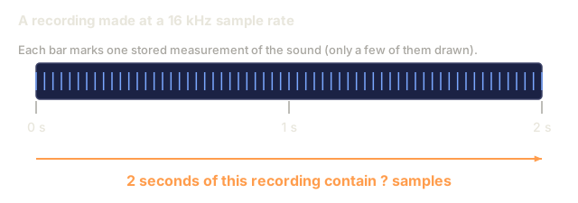
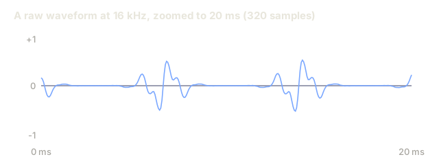
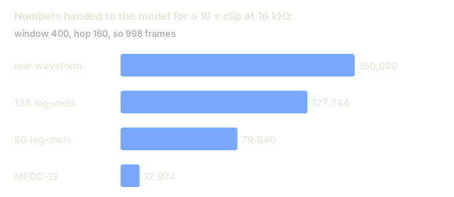
Take a 10-second clip sampled at 16 kHz. That's 160,000 floats, all sitting in [-1, 1], almost perfectly uncorrelated with the label "dog barking" or "the word cat". The information is in there, just not in a form a model can pull out directly: two identical phonemes spoken 100 ms apart produce completely different raw samples.
A spectrogram fixes that. It throws away the temporal detail human hearing never uses anyway (jitter at the microsecond scale) and keeps the structure perception actually tracks: which frequencies carry energy, over windows of roughly 10–25 ms.
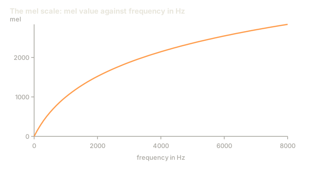
Mel spectrograms take it further. Humans perceive pitch on a log scale, so 100 Hz vs 200 Hz feels like the same gap as 1000 Hz vs 2000 Hz. The mel scale warps the frequency axis to match that perception. A mel-scaled spectrogram has been the single most important feature in speech ML from 2010 through 2026.
The Concept

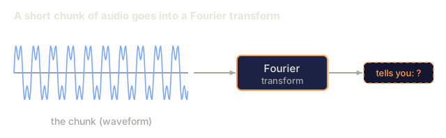
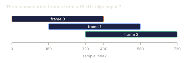
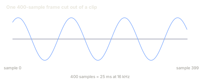
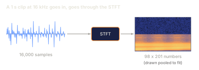
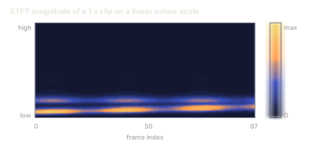
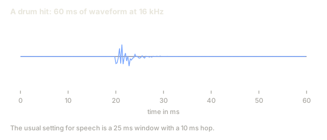
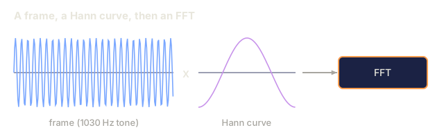
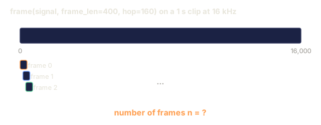
STFT (Short-Time Fourier Transform). Slice the waveform into overlapping frames (typical: 25 ms window, 10 ms hop, which is 400 samples / 160 samples at 16 kHz). Multiply each frame by a window function (Hann by default; Hamming trades off slightly differently). FFT each frame, then stack the magnitude spectra into a matrix of shape (n_frames, n_freq_bins). That matrix is your spectrogram.
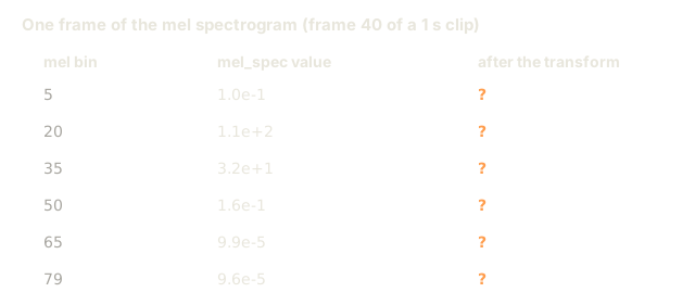
Log-magnitude. Raw magnitudes span 5-6 orders of magnitude, so every production pipeline compresses that range before doing anything else: log(|X| + 1e-6) or 20 * log10(|X|), log-magnitude rather than raw.
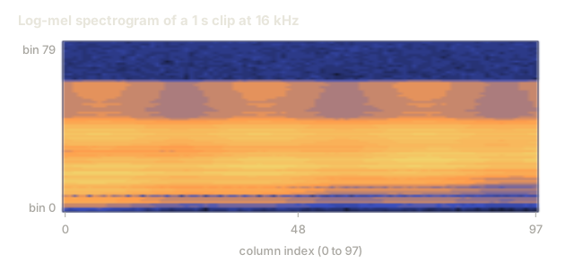
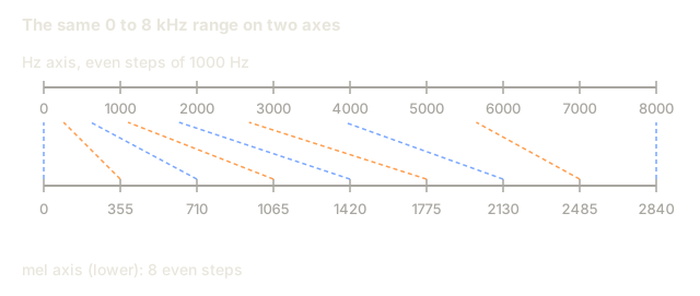
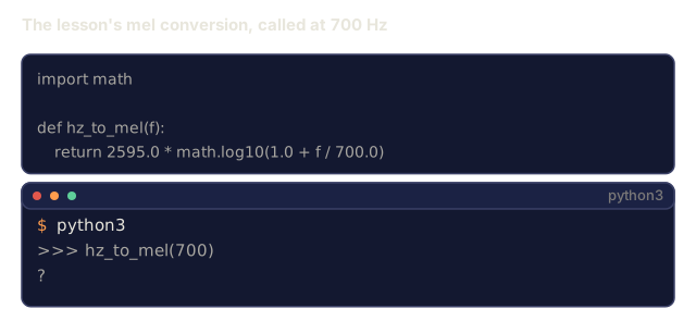
Mel scale. Frequency f in Hz maps to mel m by m = 2595 * log10(1 + f / 700). The mapping runs roughly linear below 1 kHz and roughly logarithmic above it. 80 mel bins covering 0–8 kHz is the standard ASR input.
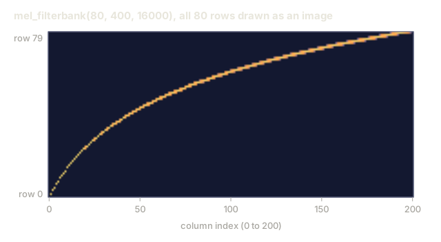
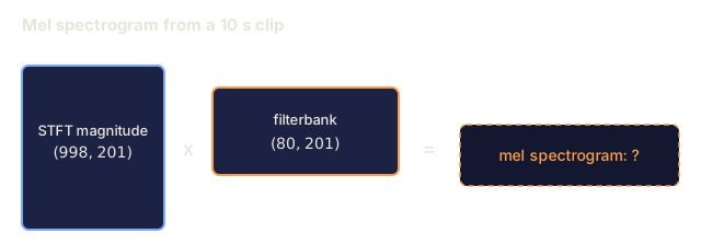
Mel filterbank. A set of triangular filters spaced equally on the mel scale, each one a weighted sum of adjacent FFT bins. Multiply the STFT magnitude by the filterbank matrix and you get the mel spectrogram in one matmul.
Log-mel spectrogram. log(mel_spec + 1e-10). Whisper, Parakeet, and SeamlessM4T all take this as input: the universal 2026 audio frontend.
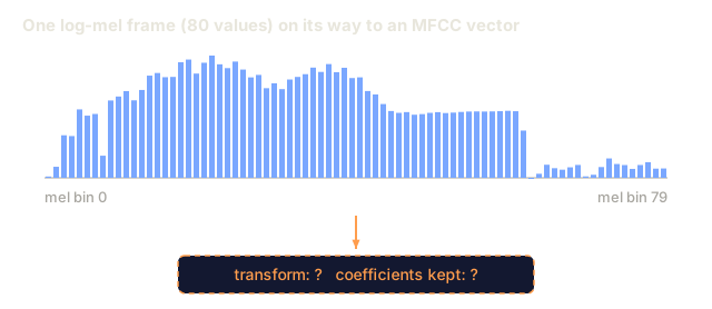
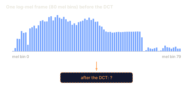
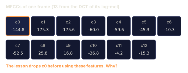
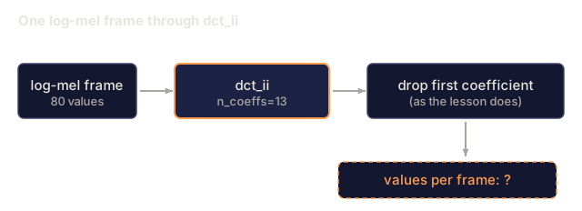
MFCCs. Take the log-mel spectrogram, apply a DCT (type II), and keep the first 13 coefficients. That decorrelates the features and compresses them further. It was the dominant feature until around 2015, when CNNs and Transformers running on raw log-mels caught up, though it still shows up in speaker recognition (x-vectors, ECAPA).
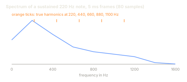
Resolution trade. A larger FFT buys better frequency resolution at the cost of worse time resolution. 25 ms / 10 ms is the audio-ML default; 50 ms / 12.5 ms fits music better; 5 ms / 2 ms is for transient detection (drum hits, plosives).
Build It
Step 1: frame the waveform
def frame(signal, frame_len, hop):
    n = 1 + (len(signal) - frame_len) // hop
    return [signal[i * hop : i * hop + frame_len] for i in range(n)]
A 10-second 16 kHz clip with frame_len=400, hop=160 yields 998 frames.
Step 2: Hann window
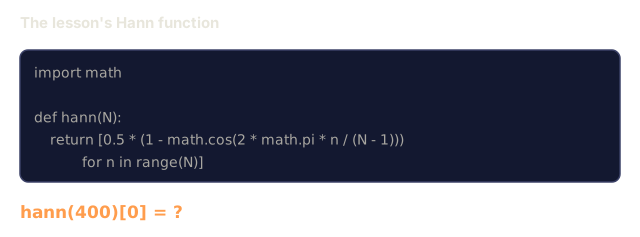
import math

def hann(N):
    return [0.5 * (1 - math.cos(2 * math.pi * n / (N - 1))) for n in range(N)]
Multiply this into each frame element-wise before the FFT. It removes the spectral leakage that comes from truncating a frame at non-zero endpoints.
Step 3: STFT magnitude
def stft_magnitude(signal, frame_len=400, hop=160):
    win = hann(frame_len)
    frames = frame(signal, frame_len, hop)
    return [magnitudes(dft([w * s for w, s in zip(win, f)])) for f in frames]
Production code uses torch.stft or librosa.stft (FFT-backed, vectorized). The loop above is pedagogical; it runs fine on the short clips in code/main.py.
Step 4: mel filterbank
def hz_to_mel(f):
    return 2595.0 * math.log10(1.0 + f / 700.0)

def mel_to_hz(m):
    return 700.0 * (10 ** (m / 2595.0) - 1)

def mel_filterbank(n_mels, n_fft, sr, fmin=0, fmax=None):
    fmax = fmax or sr / 2
    mels = [hz_to_mel(fmin) + (hz_to_mel(fmax) - hz_to_mel(fmin)) * i / (n_mels + 1)
            for i in range(n_mels + 2)]
    hzs = [mel_to_hz(m) for m in mels]
    bins = [int(h * n_fft / sr) for h in hzs]
    fb = [[0.0] * (n_fft // 2 + 1) for _ in range(n_mels)]
    for m in range(n_mels):
        for k in range(bins[m], bins[m + 1]):
            fb[m][k] = (k - bins[m]) / max(1, bins[m + 1] - bins[m])
        for k in range(bins[m + 1], bins[m + 2]):
            fb[m][k] = (bins[m + 2] - k) / max(1, bins[m + 2] - bins[m + 1])
    return fb
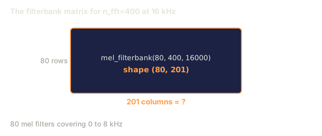
80 mels covering 0–8 kHz with n_fft=400 gives an (80, 201) matrix. Multiply the (n_frames, 201) STFT magnitude by its transpose and you get an (n_frames, 80) mel spectrogram.
Step 5: log-mel
def log_mel(mel_spec, eps=1e-10):
    return [[math.log(max(v, eps)) for v in frame] for frame in mel_spec]
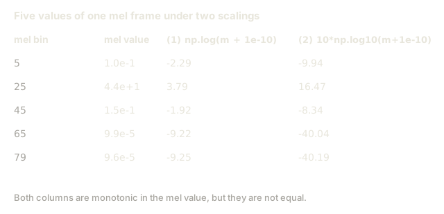
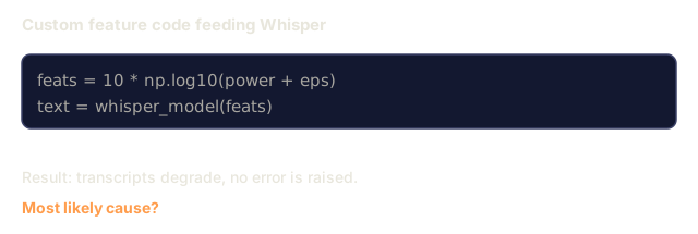
Common alternatives: librosa.power_to_db (reference-normalized dB), 10 * log10(power + eps). Whisper uses a more involved clip-and-normalize routine (see Whisper's log_mel_spectrogram).
Step 6: MFCCs
def dct_ii(x, n_coeffs):
    N = len(x)
    return [
        sum(x[n] * math.cos(math.pi * k * (2 * n + 1) / (2 * N)) for n in range(N))
        for k in range(n_coeffs)
    ]
Apply DCT to each log-mel frame and keep the first 13 coefficients. That's your MFCC matrix. The first coefficient is usually dropped, since it just encodes overall energy.
Use It
The 2026 stack:
| Task | Features |
|---|---|
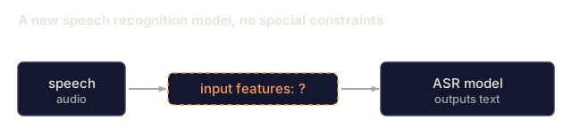
| ASR (Whisper, Parakeet, SeamlessM4T) | 80 log-mels, 10 ms hop, 25 ms window |
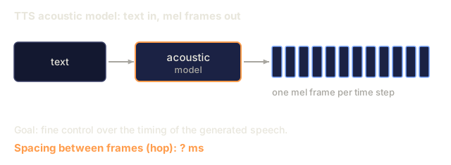
| TTS acoustic model (VITS, F5-TTS, Kokoro) | 80 mels, 5–12 ms hop for fine temporal control |
| Audio classification (AST, PANNs, BEATs) | 128 log-mels, 10 ms hop |
| Speaker embedding (ECAPA-TDNN, WavLM) | 80 log-mels or raw-waveform SSL |
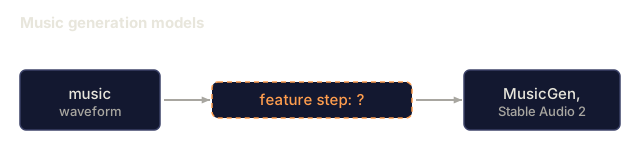
| Music (MusicGen, Stable Audio 2) | EnCodec discrete tokens (not mels) |
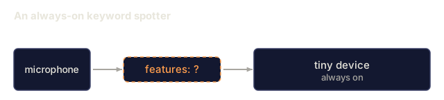
| Keyword spotting | 40 MFCCs for tiny devices |
Rule of thumb: if you are not working on music, start with 80 log-mels. The burden of proof is on any deviation.
Pitfalls that still ship in 2026
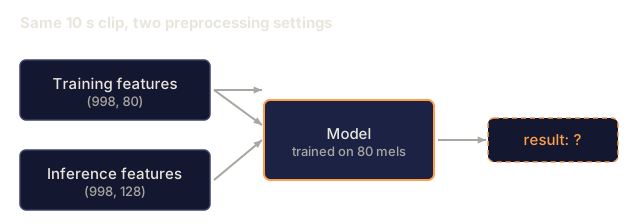
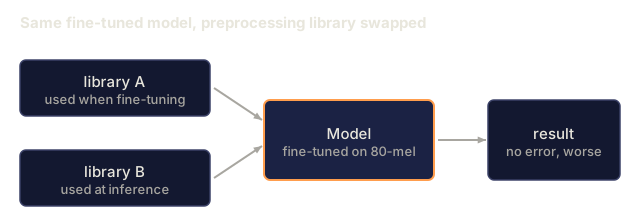
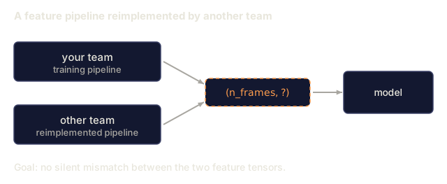
- Mel count mismatch. Train on 80 mels, run inference on 128, and nothing crashes. It just fails silently. Log the feature shape on both ends and catch it before it costs you a debugging session.
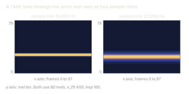
- Sample-rate mismatch upstream. Mels computed at 22.05 kHz don't look like mels computed at 16 kHz. Fix the sample rate before featurization, not after.
- dB vs log. Whisper expects log-mel, not dB-mel. A few HF pipelines autodetect the difference; your custom code will not.
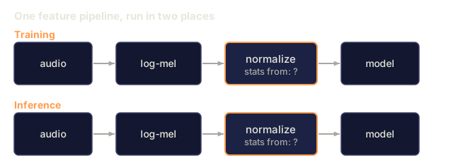
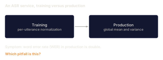
- Normalization drift. Per-utterance normalization during training, global normalization during inference: a production bug that quietly doubles WER (word error rate, the standard ASR accuracy metric).
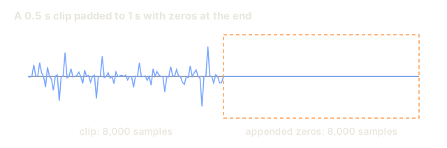
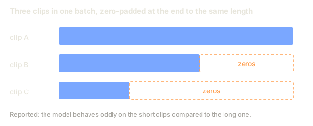
- Leakage from padding. Zero-padding the end of a clip leaves a flat spectrum in the trailing frames. Pad symmetrically, or replicate instead.
Ship It
Save this as outputs/skill-feature-extractor.md. The skill picks feature type, mel count, frame/hop, and normalization for whatever model you're targeting.
The mel-count mismatch pitfall above is the one I've personally lost a day to. Fine-tune a model on 80-mel features, swap in a slightly different preprocessing library at inference time, and it quietly defaults to 128 mels. No error, no warning, just a model that suddenly performs like it forgot how to listen. If you take one habit from this lesson, make it this: log the exact shape of your feature tensor at training time, and assert it matches at inference time, every single run. It costs one line and saves you a debugging session that won't look anything like a feature-extraction bug until you're three hours into it.
Exercises
- Easy. Run
code/main.py. It synthesizes a chirp (frequency swept 200 → 4000 Hz) and prints the argmax mel bin per frame. Plot it if you want, and confirm the peak tracks the sweep. - Medium. Re-run with
n_melsin{40, 80, 128}andframe_lenin{200, 400, 800}. Measure the sharp-peak bandwidth across the time axis. Which combination resolves the chirp best? - Hard. Implement
power_to_dband compare ASR accuracy of a tiny CNN classifier on AudioMNIST using (a) raw log-mel, (b) dB-mel withref=max, (c) MFCC-13 + delta + delta-delta. Report top-1 accuracy.
Key Terms
| Term | What people say | What it actually means |
|---|---|---|
| Frame | A slice | 25 ms chunk of waveform fed to one FFT. |
| Hop | Stride | Samples between consecutive frames; 10 ms is ASR default. |
| Window | Hann/Hamming thing | Point-wise multiplier that tapers the frame edges to zero. |
| STFT | Spectrogram generator | Framed + windowed FFT; yields time × frequency matrix. |
| Mel | Warped frequency | Log-perception scale; m = 2595·log10(1 + f/700). |
| Filterbank | The matrix | Triangular filters that project STFT onto mel bins. |
| Log-mel | Whisper's input | log(mel_spec + eps); standardized in 2026. |
| MFCC | Old-school feature | DCT of log-mel; 13 coeffs, decorrelated. |
Further Reading
- Davis, Mermelstein (1980). Comparison of parametric representations for monosyllabic word recognition: the MFCC paper.
- Stevens, Volkmann, Newman (1937). A Scale for the Measurement of the Psychological Magnitude Pitch: the original mel scale.
- OpenAI Whisper: log_mel_spectrogram source. Read the reference implementation.
- librosa feature extraction docs: reference for
mfcc,melspectrogram, and hop/window. - NVIDIA NeMo audio preprocessing: the production-scale pipeline for Parakeet + Canary models.
Code
- main.py (python, 166 lines)